SpaMTP: Refinning Metabolite Annotations

Refinning m/z Metabolite Annotations with SpaMTP

This tutorial highlights how to use SpaMTP to refine m/z annotated with multiple metabolites. SpaMTP implements this in 4 different ways, with these functions:

CalculateAnnotationStatistics
RefineLipids
Pseudo_msms
Compare_msms

We will visit each in detail below.

Author: Andrew Causer

Install and Import R Libraries

First we need to import the required libraries for this analysis.

## Install SpaMTP if not previously installed
if (!require("SpaMTP"))
    devtools::install_github("GenomicsMachineLearning/SpaMTP")

#General Libraries
library(SpaMTP)
library(Cardinal)
library(Seurat)
library(dplyr)
library(tidyr)

#For plotting + DE plots
library(ggplot2)
library(EnhancedVolcano)
library(viridis)

1) Pathway-Based Refinement: `CalculateAnnotationStatistics`

This function uses correlations in pathway expression (Metabolite only, Gene only or Multi Omic based pathway information) to refine metabolite annotation. Specifically, for each annotated metabolite, the expression profiles for all known pathways associated with this metabolite are calculated. Based on spatial colocalisation between relative pathways and the given m/z mass, each metabolite is then ranked based on Pearson correlation values and the number of significant pathways associated with that metabolite.

Below we will use a public mouse liver dataset with spotted chemicals standards to demonstrate this:

spotted <- readRDS(url("https://zenodo.org/records/17289187/files/spotted_Annotated_H_Cl_Adducts.RDS?download=1"))

spotted

## An object of class Seurat 
## 1303 features across 109390 samples within 1 assay 
## Active assay: Spatial (1303 features, 0 variable features)
##  1 layer present: counts
##  1 spatial field of view present: fov

Here we have a SpaMTP Seurat object that is already processed, with m/z annotated. Meaning we have 1303 annotated m/z values. This dataset includes certain chemical compounds which were ‘spiked-in’ at known locations. We will plot these below:

metabolite_colors <- list("ATP" = "azure","ADP" = "green","Adenosine" = "yellow", "Guanine" = "red","Glutamic Acid" = "turquoise1", "Glutamine" = "chocolate1","Glutathione" = "deeppink","liver" = "black")

ImageDimPlot(spotted, group.by = "clusters", cols = metabolite_colors, dark.background = F)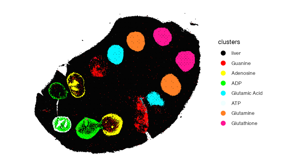

The plot highlights the location of each known metabolite. However, due to the inherent issue of mass spectrometry imaging data one m/z mass may be associated with multiple possible metabolites. For example adenosine triphosphate or ATP was spiked-in to the second set of wells within the liver (green). When we look at the annotation of ATP, we can see for m/z-505.988470137 there are 4 different annotations, one of which is ATP.

SearchAnnotations(spotted, metabolite = "Adenosine triphosphate", search.exact = T)

	raw_mz	mz_names	observed_mz	all_IsomerNames	all_Isomers	all_Isomers_IDs	all_Adducts	all_Formulas	all_Errors
1162	505.9885	mz-505.988470137	505.9885	Adenosine triphosphate; dGTP; 2-hydroxy-dATP; [[(2R,5R)-5-(6-Aminopurin-9-yl)-3,4-dihydroxyoxolan-2-yl]methoxy-hydroxyphosphoryl] phosphono hydrogen phosphate	HMDB0000538; HMDB0001440; HMDB0059593; HMDB0257997	hmdb:HMDB0000538; hmdb:HMDB0001440; hmdb:HMDB0059593; hmdb:HMDB0257997	M-H	C10H16N5O13P3	0.0019

Plotting this m/z value spatially, it localises completely within the ATP spiked-in region.

ImageDimPlot(spotted, group.by = "clusters", cols = setNames(
  ifelse(names(metabolite_colors) == "ATP", "azure", "darkgrey"),names(metabolite_colors)
))+ ggtitle("ATP")| ImageMZPlot(spotted, mzs = 505.9885)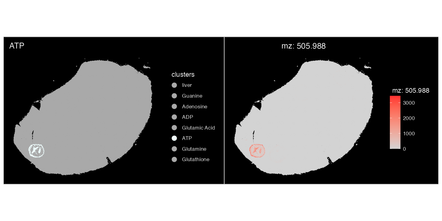

This confirms that the correct annotation of mz-505.988470137 is only ‘ATP’. This is the case with all other spiked-in chemicals. To refine the annotations based on pathway correlation we can run SpaMTP’s CalculateAnnotationStatistics:

## Step 1: Create a pathway assay - This can be done using only metabolites, or can be merged to include genes if applicable
spotted <- CreatePathwayAssay(spotted, analyte_type = "metabolites", assay = "Spatial", new_assay = "SPM_pathway", verbose = T)

## Step 2: Format Pathway Assay
DefaultAssay(spotted) <- "SPM_pathway"
spotted <- NormalizeData(spotted)
spotted <- ScaleData(spotted)

## Step 3: Run CalculateAnnotationStatistics
output <- CalculateAnnotationStatistics(data = spotted, mz.assay = "Spatial",pathway.assay="SPM_pathway", mz.slot = "counts", return.top = FALSE)

After running CalculateAnnotationStatistics the output will be a dataframe containing the most likely annotation for each m/z value based on correlations with pathway expression. Lets subset this output to look at our spiked-in metabolites:

output[c(1162,1053,501,626,126,117,251,113,248,637,638,835,836),]

	raw_mz	mz_names	metabolite	n_sig_path	max_cor	z_score	pval	pval_adj	original_annotations
1162	505.9885	mz-505.988470137	Adenosine triphosphate	2381	0.8374779	1.731981	0.0416385	0.1249154	Adenosine triphosphate; dGTP; 2-hydroxy-dATP; [[(2R,5R)-5-(6-Aminopurin-9-yl)-3,4-dihydroxyoxolan-2-yl]methoxy-hydroxyphosphoryl] phosphono hydrogen phosphate
1053	426.0221	mz-426.022139245	ADP	3579	0.8985871	2.541858	0.0055132	0.0275662	Adenosine 3’,5’-diphosphate; dGDP; ADP; [(2S,3R,4R,5R)-5-(6-Aminopurin-9-yl)-3,4-dihydroxyoxolan-2-yl]methyl phosphono hydrogen phosphate; Zidovudine diphosphate
501	266.0895	mz-266.089477461	Adenosine	104	0.9071216	3.756311	0.0000862	0.0006897	3’-Azido-3’-deoxythymidine, 98%; 8-Oxo-2’-deoxyadenosine; Adenosine; Deoxyguanosine; Vidarabine; Zidovudine; 9-Arabinofuranosyladenine; Formycin A
626	302.0662	mz-302.066155193	Adenosine	104	0.8019030	4.117214	0.0000192	0.0001726	Hpmpa; 3’-Azido-3’-deoxythymidine, 98%; 8-Oxo-2’-deoxyadenosine; Adenosine; Deoxyguanosine; Vidarabine; Zidovudine; 9-Arabinofuranosyladenine; Formycin A
126	150.0421	mz-150.042133345	Guanine	42	0.6453926	3.000000	0.0013499	0.0053996	8-Oxo-7,8-dihydrodeoxyguanine; Guanine; 2-Hydroxyadenine; 8-Hydroxyadenine
117	146.0459	mz-146.045881333	L-Glutamic acid	373	0.8193504	4.792862	0.0000008	0.0000099	N-lactoyl-Glycine; 5-Hydroxy-4-oxo-L-norvaline; Alanine acetate; N-Methyl-DL-aspartic acid; L-Glutamic acid; N-Methyl-D-aspartic acid; N-Acetylserine; O-Acetylserine; D-Glutamic acid; L-4-Hydroxyglutamate semialdehyde; 3-(Carboxymethylamino)propanoic acid; DL-Glutamate
251	182.0226	mz-182.022559065	L-Glutamic acid	343	0.2866179	5.439546	0.0000000	0.0000004	Fosmidomycin; 2-Amino-4-phosphonobutyric acid; N-lactoyl-Glycine; 5-Hydroxy-4-oxo-L-norvaline; Alanine acetate; N-Methyl-DL-aspartic acid; L-Glutamic acid; N-Methyl-D-aspartic acid; N-Acetylserine; O-Acetylserine; D-Glutamic acid; L-4-Hydroxyglutamate semialdehyde; 3-(Carboxymethylamino)propanoic acid; DL-Glutamate
113	145.0619	mz-145.061865745	L-Glutamine	137	0.5805269	4.103823	0.0000203	0.0001626	Alanylglycine; Cyclic Urea; Glycyl-D-Alanine; Glycylsarcosine; D-Alanyl glycine; L-Glutamine; Ureidoisobutyric acid; D-Glutamine; 3-ureido-isobutyrate
248	181.0385	mz-181.038543477	L-Glutamine	137	0.5005050	4.126675	0.0000184	0.0001472	Alanylglycine; Cyclic Urea; Glycyl-D-Alanine; Glycylsarcosine; D-Alanyl glycine; L-Glutamine; Ureidoisobutyric acid; D-Glutamine; 3-ureido-isobutyrate
637	306.0765	mz-306.076529999	Glutathione	175	0.7969612	4.082483	0.0000223	0.0001337	Glutathione; Glutathionate(1-); Methyl 2-((3,4-dihydro-3,4-dioxo-1-naphthalenyl)amino)benzoate; Hallacridone; Aristolodione; zaprinast
638	306.0772	mz-306.077181461	Glutathione	175	0.7969960	4.082483	0.0000223	0.0001337	Glutathione; Glutathionate(1-); Methyl 2-((3,4-dihydro-3,4-dioxo-1-naphthalenyl)amino)benzoate; Hallacridone; Aristolodione; zaprinast
835	342.0532	mz-342.053207731	Glutathione	175	0.5391956	4.082483	0.0000223	0.0001337	O-Desmethylindomethacin; Glutathione; Glutathionate(1-); Methyl 2-((3,4-dihydro-3,4-dioxo-1-naphthalenyl)amino)benzoate; Hallacridone; Aristolodione
836	342.0539	mz-342.053859193	Glutathione	175	0.5441561	4.082483	0.0000223	0.0001337	O-Desmethylindomethacin; Glutathione; Glutathionate(1-); Methyl 2-((3,4-dihydro-3,4-dioxo-1-naphthalenyl)amino)benzoate; Hallacridone; Aristolodione

We can see for each spiked-in metabolite the predicted metabolite with the highest significance in each case corresponded to the spike-in. This method gives the user higher confidence that the annotations of m/z value are correct and biologically significant. Note: For large datasets this function can take a while to run, the function CalculateSingleAnnotationStatistics can be used instead to calculate refined annotations for a single m/z value. Please visit the documentation for more information.

As described previously in the Spatial Metabolomics Analysis tutorial, because many different kinds of lipids can share the same molecular weight, this may results in some m/z values possessing many possible annotations. The SpaMTP function RefineLipids can be used to simplify the lipid nomenclature into common lipid categories and classes, giving more simplified annotations to a level that most SM datasets are capable of identifying.

### Runs lipid nomenclature simplification on annotations
refined_lipid_annotations <- RefineLipids(spotted@assays$Spatial@meta.data, annotation.column = "all_IsomerNames", lipid_info = "simple")

We can count the number of metabolites assigned for each m/z before and after refining the lipid annotations.

## Count original number of annotations per m/z 
refined_lipid_annotations <- refined_lipid_annotations %>%
  mutate(base_count = sapply(strsplit(all_IsomerNames, ";\\s*"), length))

## Count number of annotations per m/z following lipid simplification
refined_lipid_annotations <- refined_lipid_annotations %>%
  mutate(
    refined_count = ifelse(
      is.na(Lipid.Maps.Category),
      base_count,
      sapply(strsplit(Lipid.Maps.Category, ";\\s*"), length)
    )
  )

The maximum reduction in annotations was from 161 to 1. This is quite a significant simplification which can help in processing large datasets. Lets visualise the difference between each m/z value below:

# reshape to long format
df_long <- refined_lipid_annotations %>%
  select(raw_mz, refined_count, base_count) %>%
  pivot_longer(cols = c(refined_count, base_count),
               names_to = "Type", values_to = "Count")

# plot
ggplot(df_long, aes(x = raw_mz, y = Count, color = Type)) +
  geom_point(size = 2, alpha = 0.7) +
  geom_smooth(method = "lm", se = FALSE, size = 1.2) +
  scale_color_manual(values = c("refined_count" = "red",
                                "base_count" = "blue"),
                     labels = c("Base annotations", "Refined annotations")) +
  labs(
    x = expression(italic("m/z")),
    y = "Number of annotations",
    color = ""
  ) +
  theme_minimal(base_size = 14) +
  theme(
    legend.position = "top",
    panel.grid.minor = element_blank(),
    axis.title = element_text(face = "bold")
  )

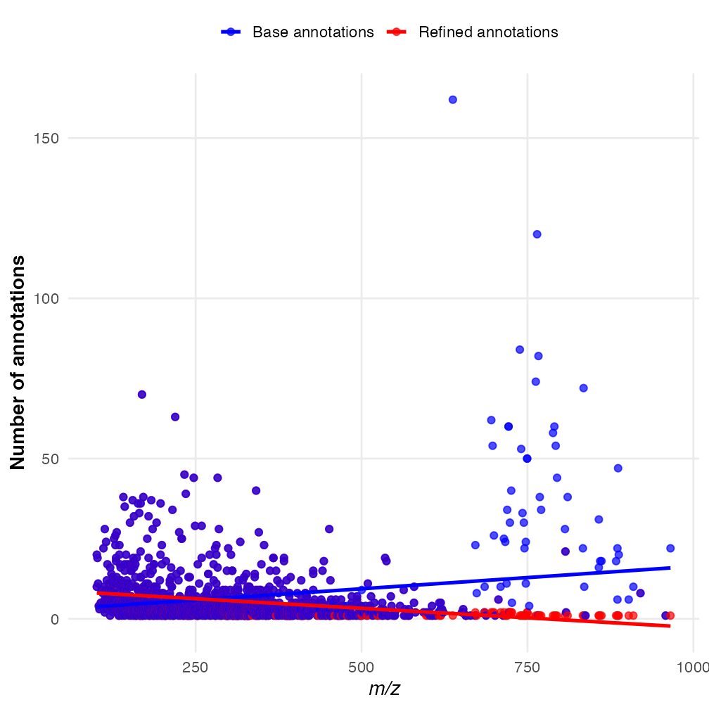
We can see the larger m/z values, which correspond mostly to lipids, display the biggest differences following annotation refinement.

To come!

Refinning m/z Metabolite Annotations with SpaMTP

Install and Import R Libraries

1) Pathway-Based Refinement: `CalculateAnnotationStatistics`

2) Lipid Nomenchlature Refinement

3) Pseudo MS/MS-Based Refinement

4) Refinement with Paired Targeted Metabolic Data

SpaMTP: Refinning Metabolite Annotations

Refinning m/z Metabolite Annotations with SpaMTP

Install and Import R Libraries

1) Pathway-Based Refinement: CalculateAnnotationStatistics

2) Lipid Nomenchlature Refinement

3) Pseudo MS/MS-Based Refinement

4) Refinement with Paired Targeted Metabolic Data

1) Pathway-Based Refinement: `CalculateAnnotationStatistics`