SpaMTP: Spatial Multi-Omics Analysis
Source:vignettes/Multi-Omic_Mouse_Brain.Rmd
Multi-Omic_Mouse_Brain.RmdMulti-Omics Mouse Brain Vignette
This tutorial highlights the utility of SpaMTP on
multi-omic data. This vignette will use mouse brain data, where both
Spatial Transcriptomics (Visium), ST, and Spatial Metabolomics
(MALDI-MSI), SM, were generated from the same tissue section. This data
is publicly available from Vicari et al and all
data objects used for this vignette are available from the SpaMTP
zenodo page.
Using SpaMTP we will highlight:
- Loading SM Data
- Manually Aligning SM and ST datasets
- Mapping Aligned SM data to ST Spot Level
- Multi-Modal Data Integration of SM and ST Data
- Multi-Omic Data Visualisation
- Co-localisation of Metabolites and Genes
- Multi-Modality Pathway Analysis
Author: Andrew Causer
Load Data
Here, we will load in both our Visium and MALDI-MSI data! The Visium data is contained in 10X Genomic’s standard format. The MALDI-MSI data is in a matrix format, where one table contains both x and y coordinates, and also intensity values for each m/z value.
Install and Import R Libraries
First, we need to import the required libraries for this analysis:
## Install SpaMTP if not previously installed
if (!require("SpaMTP"))
devtools::install_github("GenomicsMachineLearning/SpaMTP")
#General Libraries
library(SpaMTP)
library(Cardinal)
library(Seurat)
library(dplyr)
#For plotting + DE plots
library(ggplot2)
library(EnhancedVolcano)
library(mclust)
library(patchwork)
## For reproducability
set.seed(888)Load SM Data
As mentioned above, the format of our SM data is in a mtx format. This is different to .ibd and .imzML files that were used in the Spatial Metabolomics Analysis: Mouse Bladder Vignette. The layout of this dataset is demonstrated below:
| x | y | mz_1 | mz_2 | mz_3 | … | mz_n |
|---|---|---|---|---|---|---|
| 0 | 1 | 0 | 0 | 11 | … | 0 |
| 0 | 2 | 0 | 0 | 0 | … | 0 |
| 0 | 3 | 15 | 0 | 0 | … | 32 |
| 0 | 4 | 20 | 0 | 0 | … | 32 |
| 0 | 5 | 0 | 20 | 0 | … | 0 |
Based on this, we can read in the .csv file that
contains our intensity and pixel coordinate values.
# Load directly from file
#msi <- ReadSM_mtx("./V11L12-109_B1.Visium.FMP.220826_smamsi.csv")
# Load directly from URL
msi_url <- "https://zenodo.org/records/17246900/files/V11L12-109_B1.Visium.FMP.220826_smamsi.csv?download=1"
msi <- ReadSM_mtx(mtx.file = msi_url)Spliting matrix data from column 1 onwards ....
Adding Pixel Metadata ....
Creating Centroids for Spatial Seurat Object ....Great! Now lets explore our sample. First, we will see the layout of the SpaMTP Seurat Object:
msi## An object of class Seurat
## 1538 features across 4914 samples within 1 assay
## Active assay: Spatial (1538 features, 0 variable features)
## 1 layer present: counts
## 1 spatial field of view present: fovWe can see that we have about 1,538 different m/z masses across 4,914 pixels.
Lets look at what we have in our metadata!
head(msi@meta.data)| orig.ident | nCount_Spatial | nFeature_Spatial | x_coord | y_coord | |
|---|---|---|---|---|---|
| 0_0 | 0 | 0 | 0 | 0 | 0 |
| 0_1 | 0 | 0 | 0 | 0 | 1 |
| 0_2 | 0 | 0 | 0 | 0 | 2 |
| 0_3 | 0 | 0 | 0 | 0 | 3 |
| 0_4 | 0 | 0 | 0 | 0 | 4 |
| 0_5 | 0 | 0 | 0 | 0 | 5 |
We can see that our pixel names are a combination of x and y coordinates. We also have two data columns, nCount_Spatial and nFeature_Spatial, were were generated when loading the data. Respectively, these represent the total intensity across all m/z per pixel, and the number of different m/z values which have an intensity > 0 per pixel.
Lets have a look at the sample spatially. We will just visualise the number of m/z’s per pixel.
ImageFeaturePlot(msi, "nFeature_Spatial", size = 2, dark.background = FALSE) ## Warning: `aes_string()` was deprecated in ggplot2 3.0.0.
## ℹ Please use tidy evaluation idioms with `aes()`.
## ℹ See also `vignette("ggplot2-in-packages")` for more information.
## ℹ The deprecated feature was likely used in the Seurat package.
## Please report the issue at <https://github.com/satijalab/seurat/issues>.
## This warning is displayed once every 8 hours.
## Call `lifecycle::last_lifecycle_warnings()` to see where this warning was
## generated.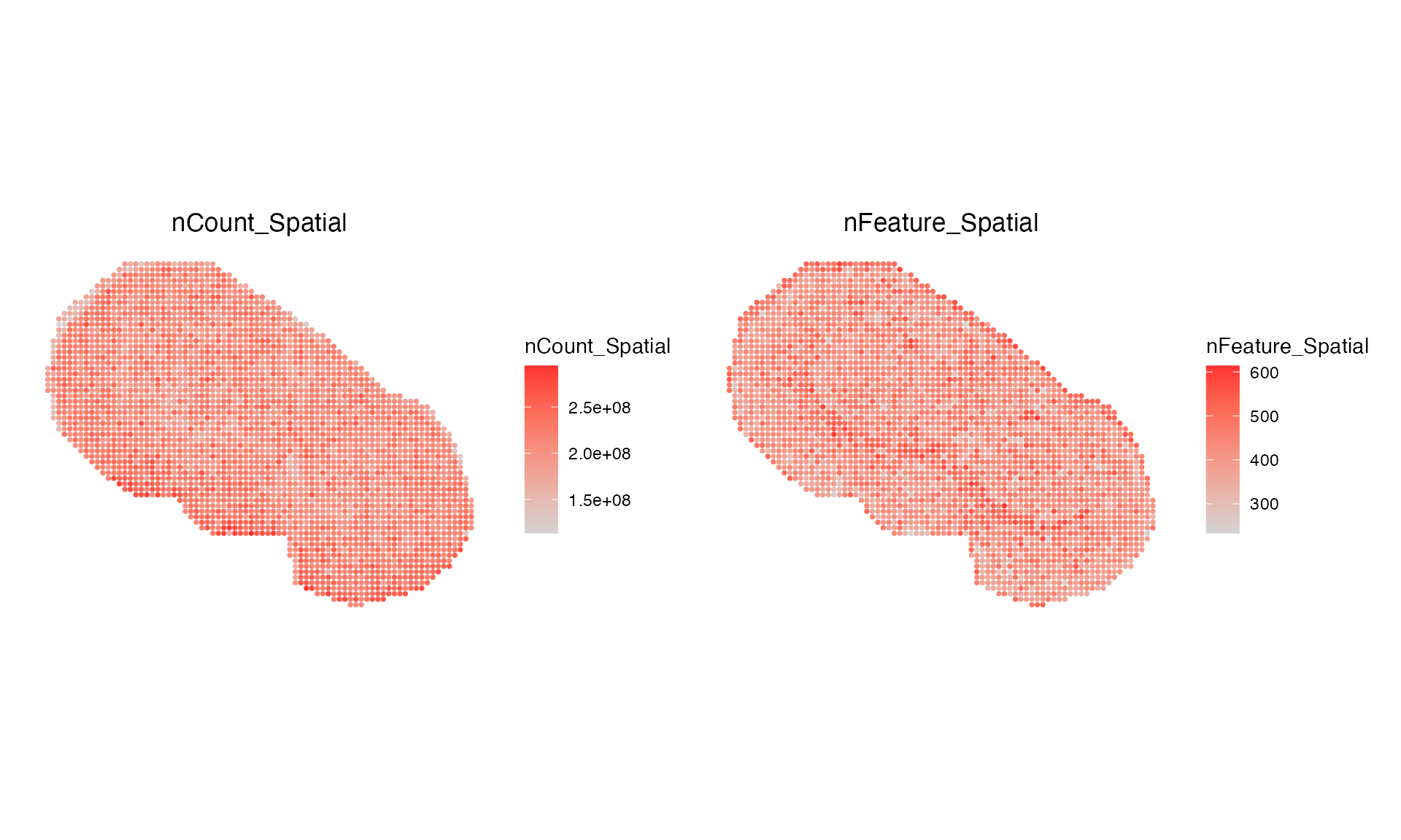
We have some pixels which do not contain any SM data, thus we will remove them first before starting any analysis.
msi <- subset(msi, subset = nCount_Spatial > 0)
ImageFeaturePlot(msi, "nCount_Spatial", size = 1.3, dark.background = FALSE) | ImageFeaturePlot(msi, "nFeature_Spatial", size = 1.3, dark.background = FALSE)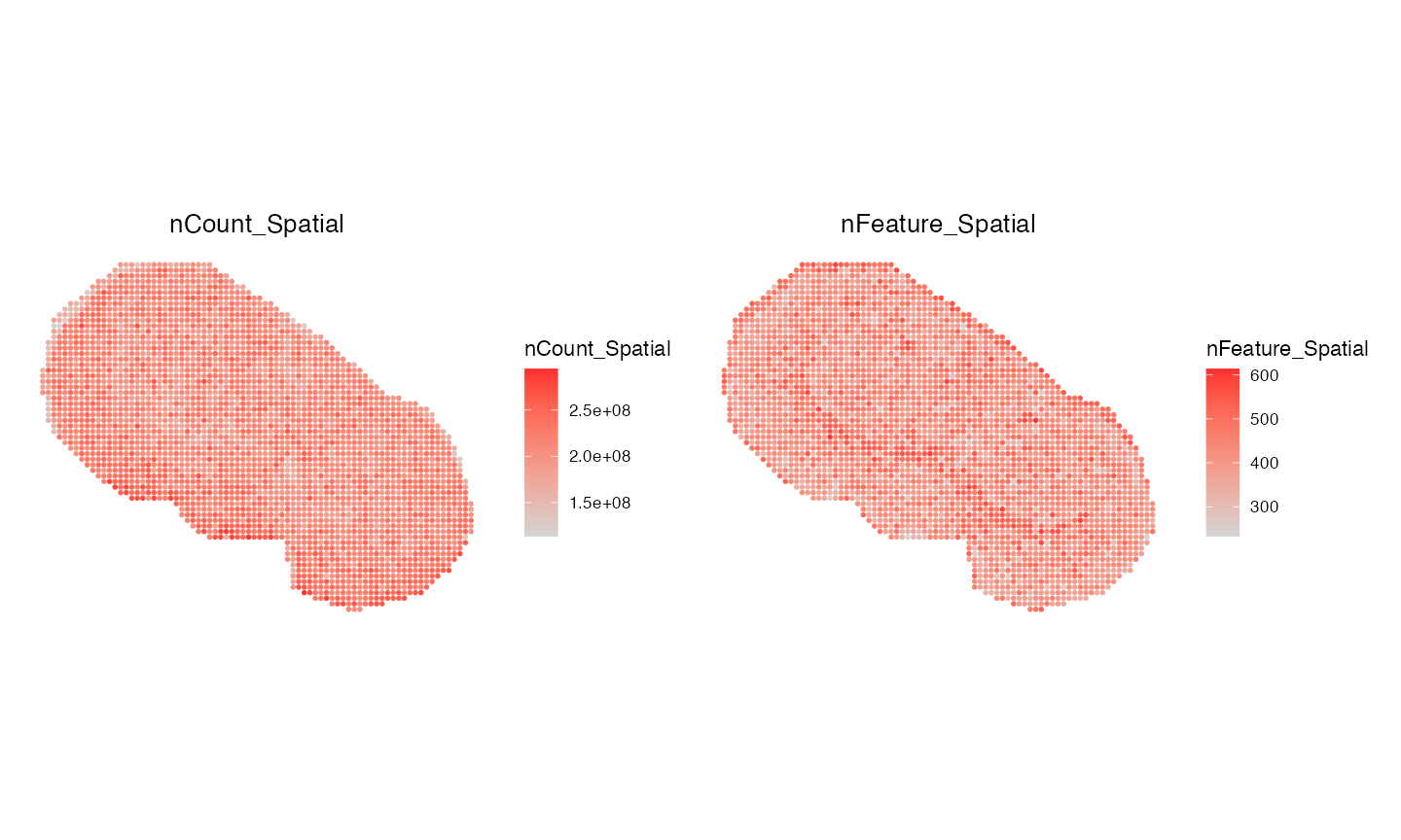
We will also change our orig.ident to sample name for
later reference:
msi@meta.data$orig.ident <- "msi_sample1"Load ST Data
Now that we have successfully loaded our SM data, lets load in the ST
Visium data. This data can be loaded using Seurat’s
Load10X_Spatial() function.
vis <- Load10X_Spatial("vignette_data_files/Mouse_Brain/ST_data/outs/")
vis ## An object of class Seurat
## 32285 features across 3120 samples within 1 assay
## Active assay: Spatial (32285 features, 0 variable features)
## 1 layer present: counts
## 1 spatial field of view present: slice1The ST data has 32,285 genes and 3,120 spots. Next, we will visualise the sample and compare to the MSI image above.
SpatialFeaturePlot(vis, features = c("nCount_Spatial", "nFeature_Spatial"), pt.size.factor = 2)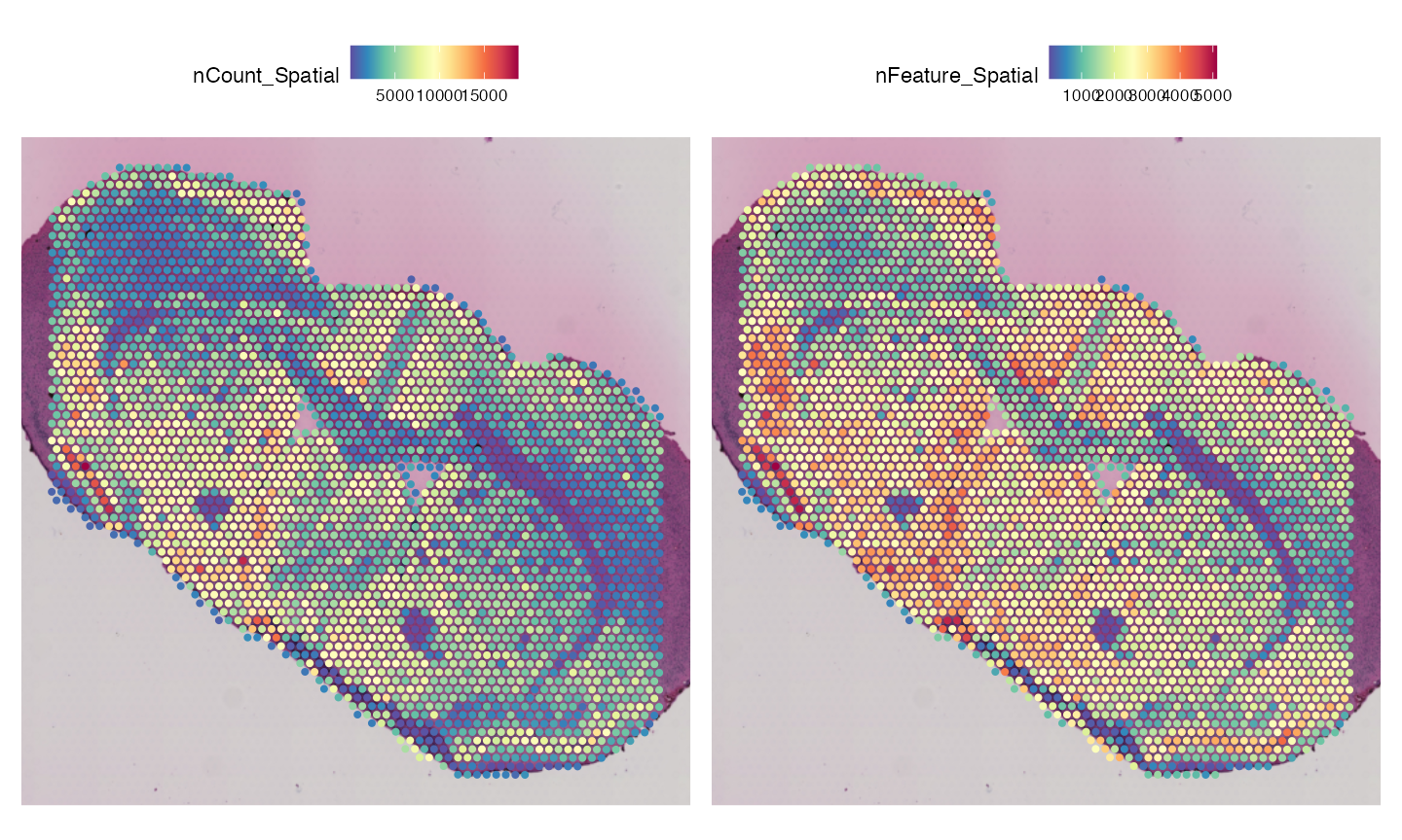
In addition, we can load in the metadata associated with the tissue morphology generated by the authors of the original publication. As mentioned previously, the data we are analysing is from a Parkinson’s mouse model, where the dopamine neurons of one brain hemisphere has been lesioned. The metadata loaded below contains information of surrounding tissue structures and the lesion site.
Now, lets load this metadata and add it to our Visium Seurat object.
## Read in metadata files
lesion <- read.csv("./outs/lesion.csv", row.names = 1)
region <- read.csv("./outs/region.csv", row.names = 1)
region_loupe <- read.csv("./outs/RegionLoupe.csv", row.names = 1)
## Combine into one dataframe
annotations <- cbind(lesion,region,region_loupe)
## Add data to metadata slot
vis@meta.data[colnames(annotations)] <- annotations[colnames(annotations)]
vis@meta.data <- vis@meta.data %>% mutate(annotations = ifelse(RegionLoupe %in% c("CP", "ACB"), paste0(RegionLoupe, "_", lesion), RegionLoupe))
head(vis)| orig.ident | nCount_Spatial | nFeature_Spatial | lesion | region | RegionLoupe | annotations | |
|---|---|---|---|---|---|---|---|
| AAACAAGTATCTCCCA-1 | SeuratProject | 3491 | 1562 | lesioned | striatum | CP | CP_lesioned |
| AAACAGCTTTCAGAAG-1 | SeuratProject | 1454 | 626 | intact | not_striatum | ||
| AAACATTTCCCGGATT-1 | SeuratProject | 5784 | 2275 | lesioned | striatum | CP | CP_lesioned |
| AAACCCGAACGAAATC-1 | SeuratProject | 2048 | 1193 | lesioned | not_striatum | CTX | CTX |
Now, we can plot the results. We can use this information later for tissue alignment and removing poor quality spots sitting outside the tissue section.
SpatialDimPlot(vis, group.by = c("lesion","region", "RegionLoupe"))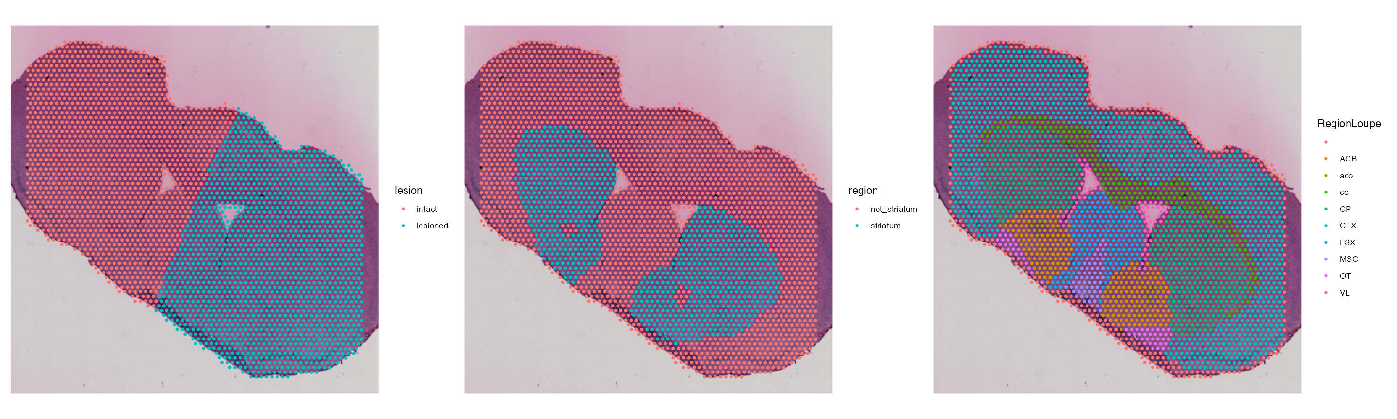
Data preprocessing
Annotate m/z masses
Now that we have successfully loaded our ST and SM data, we can now run some general pre-processing to remove any poor quality spots/pixel and genes/metabolites.
In this case, the matrix run was an FMP10 matrix, meaning some of the
masses of our metabolites have an additional mass added to their weight,
and thus require a specialised annotation database to ensure the
annotations correct for this additional mass. SpaMTP has an inbuilt
function for annotating metabolites from FMP10 matrices called
AddFMP10Annotations(). This function also allows for the
addition of custom/additional metabolites that aren’t annotated in the
current dataset.
Parkinson’s is heavily associated with dopamine regulation, and thus
we will also use the add.custom.annotations parameter to
include the annotation of this molecule.
First, we will need to load this additional data.frame containing the custom annotations:
fmp10_metabolites <- read.csv(url("https://zenodo.org/records/17246900/files/Public_data_FMP10_Annotations.csv?download=1"), row.names = 1)
fmp10_metabolites| Observed.MZ | Reference_mz | IsomerNames | Adduct | Formula | Matched.delta.mass..Da. | Error | Exactmass | mass | annotation | Isomers | Isomers_IDs |
|---|---|---|---|---|---|---|---|---|---|---|---|
| 435.21 | 435.21 | 3-Methoxytyramine (3-MT) | [M+FMP10] | C9H13NO2 | 0 | 0 | 435.21 | 435.21 | 3-Methoxytyramine (3-MT) | HMDB0000022 | hmdb:HMDB0000022 |
| 421.19 | 421.19 | Dopamine (single derivatized) | [M+FMP10] | C8H11NO2 | 0 | 0 | 421.19 | 421.19 | Dopamine (single derivatized) | HMDB0000073 | hmdb:HMDB0000073 |
| 674.28 | 674.28 | Dopamine (double derivatized) | [M+2FMP10a] | C8H11NO2 | 0 | 0 | 674.28 | 674.28 | Dopamine (double derivatized) | HMDB0000073 | hmdb:HMDB0000073 |
| 690.28 | 690.28 | Norephinephrine (NE) (double derivatized) | [M+2FMP10a] | C8H11NO3 | 0 | 0 | 690.28 | 690.28 | Norephinephrine (NE) (double derivatized) | HMDB0000216 | hmdb:HMDB0000216 |
Next, we can add these custom annotations to the FMP10 database and annotate our dataset:
msi_annotated <- AddFMP10Annotations(msi, add.custom.annotation = fmp10_metabolites, assay = "Spatial", return.only.annotated = F)If we had a specific list of annotations, regardless of the matrix
used to generate the data, we can add these custom annotations using the
AddCustomMZAnnotations() function. This function only
requires a data.frame containing two columns named mass and
annotation. We can see below how this differs from using
the inbuilt FMP10 database:
custom_panel <- fmp10_metabolites[c("mass", "annotation")]
custom_panel| mass | annotation |
|---|---|
| 435.21 | 3-Methoxytyramine (3-MT) |
| 421.19 | Dopamine (single derivatized) |
| 674.28 | Dopamine (double derivatized) |
| 690.28 | Norephinephrine (NE) (double derivatized) |
msi_custom_annotated <- AddCustomMZAnnotations(msi, custom_panel)The functions above add these annotations into the SpaMTP object’s feature meta.data slot. We can see and this below:
msi_annotated[["Spatial"]]@meta.data[413:414,]| raw_mz | mz_names | all_IsomerNames | Error | Reference_mz | true_mzs | all_Isomers | all_Isomers_IDs | all_Adducts | all_Formulas | all_Errors | |
|---|---|---|---|---|---|---|---|---|---|---|---|
| 413 | 421.1914 | mz-421.19136 | Dopamine (single derivatized) | NA | NA | 421.19136 | HMDB0000073 | hmdb:HMDB0000073 | [M+FMP10] | C8H11NO2 | 0.00135999999997694 |
| 414 | 422.1391 | mz-422.13913 | Gentisic acid; 2-Pyrocatechuic acid; Protocatechuic acid; 2,6-Dihydroxybenzoic acid; 3,5-Dihydroxybenzoic acid; 2,4-Dihydroxybenzoic acid; 2,4,6-trihydroxybenzaldehyde; 3,4,5-Trihydroxybenzaldehyde | -1.385026; -1.385042 | 422.1381 | 422.13913 | HMDB0000152; HMDB0000397; HMDB0001856; HMDB0013676; HMDB0013677; HMDB0029666; HMDB0125090; HMDB0246043 | hmdb:HMDB0000152; hmdb:HMDB0000397; hmdb:HMDB0001856; hmdb:HMDB0013676; hmdb:HMDB0013677; hmdb:HMDB0029666; hmdb:HMDB0125090; hmdb:HMDB0246043 | [M+FMP10] | C7H6O4 | 0.0010300000000143 |
msi_custom_annotated[["Spatial"]]@meta.data[413:414,]| raw_mz | mz_names | mass | all_IsomerNames | true_mzs | ppm_diff | |
|---|---|---|---|---|---|---|
| 413 | 421.1914 | mz-421.19136 | 421.19 | Dopamine (single derivatized) | 421.19136 | 0.00135999999997694 |
| 414 | 422.1391 | mz-422.13913 | No Annotation | No Annotation | No Annotation | No Annotation |
We can see that based on the FMP10-tagged value, we are able to annotated some of our m/z values with their respective metabolites.
Dopamine plays a critical part in Parkinson’s disease, so lets visualise this annotation spatially!
ImageMZAnnotationPlot(msi_annotated, "Dopamine (double derivatized)", slot = "counts", dark.background = FALSE, size = 1.5)
There is a strong localisation of dopamine in the non-lesioned hemisphere.
Align Multi-Omic Technologies
Although we have two -omic datasets from the same sample, the coordinates are not aligned in their current format. We can see this in the first plot below.
df1 <- GetTissueCoordinates(vis)
df1$sample <- "RNA"
df2 <- GetTissueCoordinates(msi_annotated)
df2[,"sample"] <- "MSI"
p1 <- ggplot(df1, aes(x, y,color = sample)) + theme_classic() + geom_point(size = 0.5) + scale_color_manual(values = "blue")
p2 <- ggplot(df2, aes(x, y,color = sample)) + theme_classic() + geom_point(size = 0.5) + scale_color_manual(values = "red")
p1|p2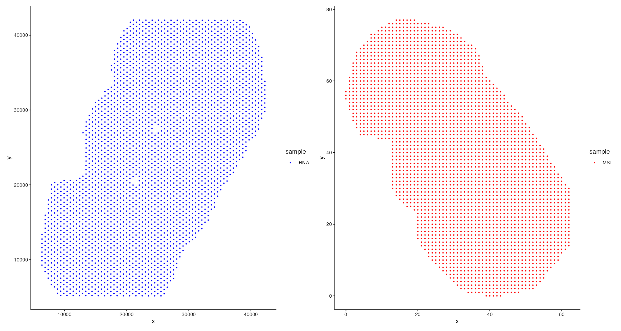
To achieve multi-omic alignment, we must perform 2 steps:
1. Align Coordinates:
- Here, we will manually adjust the coordinates of the SM data to match the H&E image of the Visium data using a Shiny app generated through ManualAlignImages()
- We can change what data is plotted/visualised to assist with correct alignment
- This will output a SM SpaMTP Seurat Class Object with transformed coordinates (transformed via an affine transformation)
2. Map Omic Data to Common Spots:
- The final step is to map or bin the SM data to each ST spot using MapSpatialOmics()
- This step works by finding all SM data points within a radius of a ST spot and assigning their respective data
- Increasing the SM resolution in this function can improve the mapping by reducing the distance between pixel and spot centroids.
Lets run these functions on our sample:
Running this code below will activate an interactive shiny app where users can align two datasets. This example can also be visualised here.
msi_transformed <- AlignSpatialOmics(sm.data = msi_annotated, st.data = vis)Loading required package: shiny
Show in New Window
Listening on http://0.0.0.0:4698
Sample: 2
1.21 4.587997e-18 73.5047
4.587997e-18 -1.21 580.6509
0 0 1 Lets observe the change to the coordinates, comparing between the
original x and y coordinates stored in our meta.data and our updated
pixel coordinates stored in the @image$fov slot:
head(msi_transformed)| orig.ident | nCount_Spatial | nFeature_Spatial | x_coord | y_coord | |
|---|---|---|---|---|---|
| 0_55 | msi_sample1 | 216796272 | 468 | 0 | 55 |
| 0_56 | msi_sample1 | 211210064 | 496 | 0 | 56 |
| 0_57 | msi_sample1 | 208775613 | 522 | 0 | 57 |
| 1_52 | msi_sample1 | 222418420 | 512 | 1 | 52 |
head(GetTissueCoordinates(msi_transformed))| x | y | cell |
|---|---|---|
| 5895.680 | 14550.70 | 0_55 |
| 5895.680 | 13965.14 | 0_56 |
| 5895.680 | 13379.58 | 0_57 |
| 6481.237 | 16291.33 | 1_52 |
| 6481.237 | 15713.79 | 1_53 |
| 6481.237 | 15128.23 | 1_54 |
We can see that the values have been up-scaled to matched with the visium coordinates.
CheckAlignment(msi_transformed, vis, image.res = NULL, size = 0.8)
We can also check that our SM coordinates haven’t been distorted by plotting a m/z value. Let’s compare the before vs after.
ImageMZPlot(msi_annotated, mzs = 674.28, size = 2, slot = "counts") |
ImageMZPlot(msi_transformed, mzs = 674.28, size = 2, slot = "counts")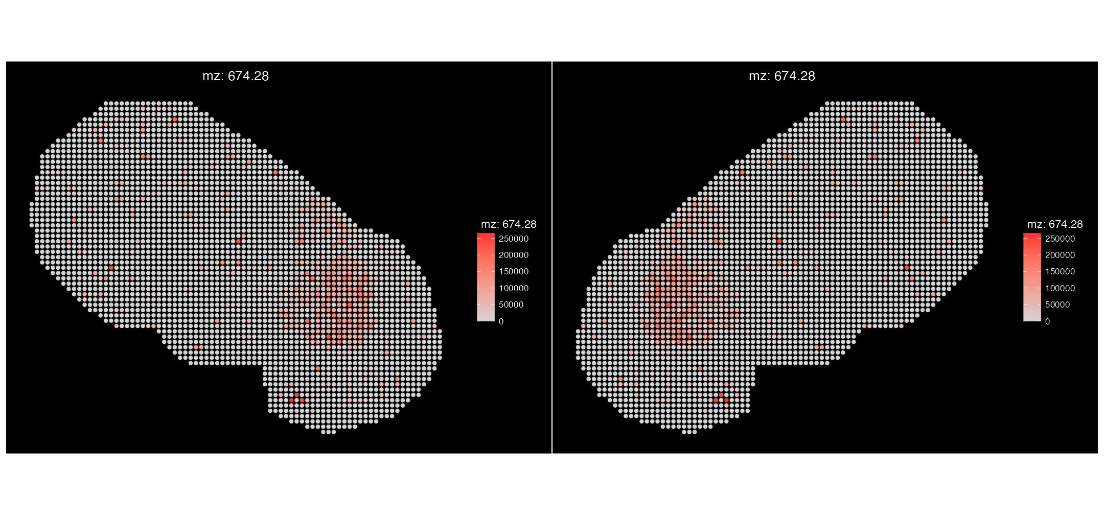
Great, now that we are confident that our SM and ST data are aligned to the same coordinates, we can map each pixel and their relative m/z intensity values to their corresponding ST spot. We have selected an overlap threshold of 30%, meaning that for a pixel to be mapped to a spot atleast 30% of its total area must be overlapping with the corresponding visium spot.
NOTE: check your version of SeuratObject, if => 5.2.0
we must update our SpaMTP Seurat Object first before running
MapSpatialOmics.
packageVersion("SeuratObject")## [1] '5.2.0'In our case we need to run UpdateSeuratObject.
msi_transformed <- UpdateSeuratObject(msi_transformed)
combined.data <- MapSpatialOmics(SM.data = msi_transformed, ST.data = vis, overlap.threshold = 0.3, annotations = TRUE, ST.scale.factor = NULL)Running `MapSpatialOmics` in lowres mode! This is normally used for bin/spot-based spatial data (Visium)...
Inputs of `ST.scale.factor`, `overlap.threshold` and `merge.unique.metadata` are required for lowres mode, please ensure they are included ...
No pixel width was provided, calculating meadian SM pixel width ...
SM pixel width used for mapping = 569.514635563575...
Generating polygon from SM pixel coordinates ...
Generating polygon from ST spot coordinates ...
Assigning SM polygons to overlapping ST polygons ...
Generating new Spatial Multi-Omic SpaMTP Seurat Object ...
Averaging SM intensity values per ST spot ...
Adding SM metadata to the new SpaMTP Seurat Object ...
Adding metabolite annotation metadata to the new SpaMTP Seurat Object ... Lets visualise how the mapping went and compare it to our original SM data object:
ImageMZPlot(msi_transformed, mzs = 674.28, size = 2, slot = "counts") |
SpatialMZPlot(combined.data, mzs = 674.28, assay = "SPM", slot = "counts", pt.size.factor = 2.2)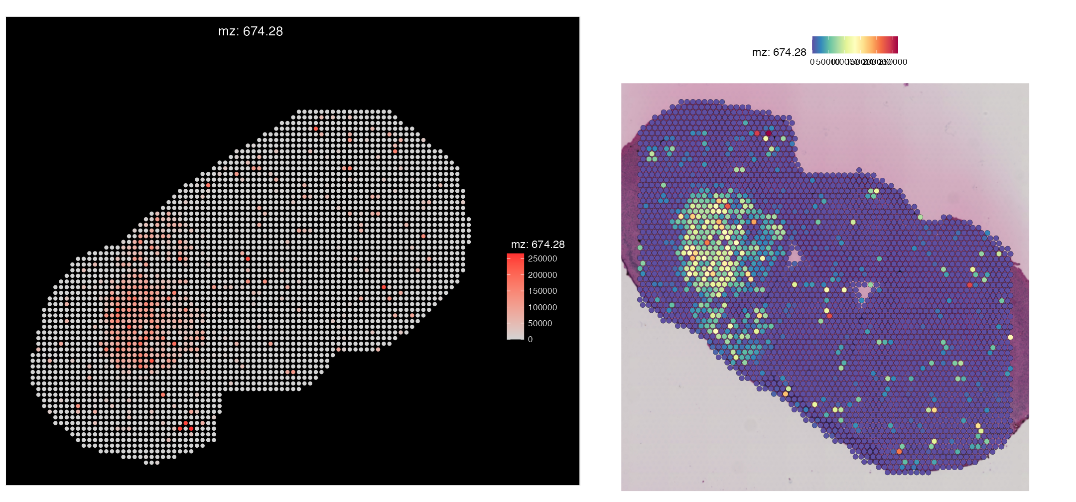
We can see that the expression of Dopamine (mz-674.28) displays the same pattern spatially in our Visium mapped object, compared to the original MSI-only data object.
Our data is almost ready for downstream analyses. However, based on the provided annotations displayed above, we should remove all spots that are not annotated as an anatomical region (meaning they are located outside of the tissue).
combined.data <- subset(combined.data, subset = RegionLoupe == "", invert = T)
SpatialDimPlot(combined.data, group.by = c("lesion", "RegionLoupe"), pt.size.factor = 2)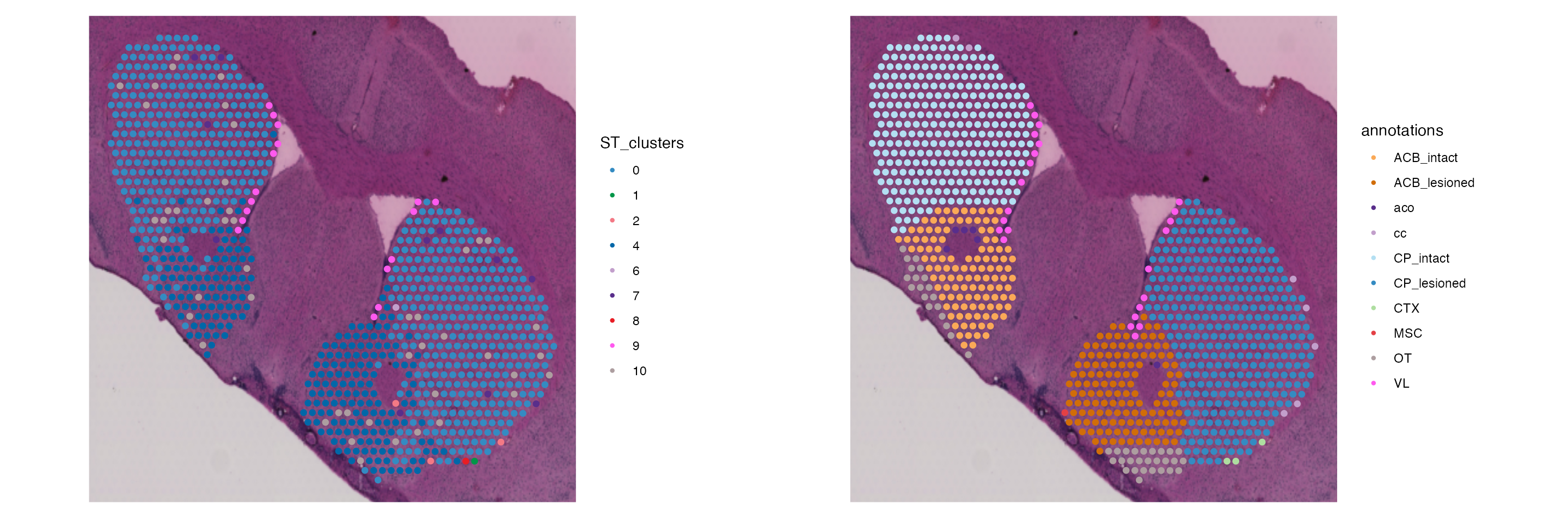
We can now see that we have removed spots that were associated with the outer border of the tissue. For example, the bottom portion of this section has a fold in the H&E and thus is technical noise, meaning these spots need to be removed.
Clustering/Downstream Analysis
Now that our spatial datasets are cleaned and fully aligned, we can perform some downstream analyses to determine cell types, differentially expressed genes and metabolites, and also upregulated metabolic pathways.
Note: Hidden below are the colour palettes used to plot.Colour Palettes
annotation_palette <- list("ACB_intact" = "#faa957", "ACB_lesioned" = "#d16d08", "aco" = "#592e8b","cc" = "#c29fcb", "CP_intact" = "#b3dff2" ,"CP_lesioned" = "#348bc2","CTX" = "#aedea0","LSX" = "#f37985", "MSC" = "#e34045", "OT" = "#ad9ea0","VL" = "#ff59ee")
# Non-Spatial Palettes
SM_palette <- list("0" = "#9dce71", "1" = "#009648", "2" = "#348bc2", "3" = "#b3dff2", "4" = "#c29fcb")
ST_palette <- list("0" = "#348bc2", "1" = "#009648", "2" = "#f37985","3" = "#fcf283", "4" = "#0067a8" , "5" = "#9dce71", "6" = "#c29fcb", "7" = "#592e8b","8" = "#e81d25","9" = "#ff59ee","10" = "#ad9ea0")
# Spatial Palettes
intergrated_palette <- list("0" = "#9dce71", "1" = "#338bc3", "2" = "#b4dff1","3" = "#e62127", "4" = "#f37985" , "5" = "#009648", "6" = "#c2a0cb", "7" = "#b0d8a0","8" = "#d16e28","9" = "#592e8a","10" = "#faaa59", "11" = "#fcf286")
spatial_SM_palette <- list("1" = "#b4dff1", "2" = "#fcf286", "3" = "#009648", "4" = "#b0d8a0", "5" = "#faaa59", "6"= "#f37985", "7" = "#338bc3","8"= "#338bc3", "9"= "#cc6dab", "10"="#c2a0cb", "11"="#592e8a")
spatial_ST_palette <- list("1" = "#cc6dab", "2" = "#c2a0cb", "3" = "#f37985" ,"4" = "#9dce71", "5" = "#b4dff1", "6" = "#e62127", "7" = "#338bc3","8" = "#009648","9" = "#0068a8","10" = "#fcf286","11" = "#592e8a")Seurat-Based Clustering
As previously demonstrated in the Spatial
Metabolomics Analysis Vignette, we can use functions already
implemented by Seurat for performing unsupervised
clustering on not only ST data, but also metabolic data.
Cluster ST data
First, we will run clustering on the ST data. Based on the two different modalities, mRNA data will perform much better at defining different cell types/structures within the tissue sample. We expect the clustering to be able to detect cell types/regions, such as the striatum.
DefaultAssay(combined.data) <- "SPT"
## Run ST clustering
combined.data <- NormalizeData(combined.data, verbose = FALSE)
combined.data <- FindVariableFeatures(combined.data, verbose = FALSE)
combined.data <- ScaleData(combined.data, verbose = FALSE)
combined.data <- RunPCA(combined.data, npcs = 30, reduction.name = "spt.pca", verbose = FALSE)
combined.data <- FindNeighbors(combined.data, dims = 1:30, reduction = "spt.pca", verbose = FALSE)
combined.data <- RunUMAP(combined.data, dims = 1:30, reduction = "spt.pca", reduction.name = "spt.umap", verbose = FALSE)
combined.data <- FindClusters(combined.data, resolution = 0.5, cluster.name = "ST_clusters", verbose = FALSE)
DimPlot(combined.data, group.by = "ST_clusters", reduction = "spt.umap", cols = ST_palette) |
SpatialDimPlot(combined.data, group.by = "ST_clusters", pt.size.factor = 2.1, cols = ST_palette)
The clustering results demonstrate clear groups of cells. Lets compare them to the provided annotations:
striatum <- subset(combined.data, subset = region == "striatum")
SpatialDimPlot(striatum, group.by = "ST_clusters", label = F, pt.size.factor = 2.4, cols = ST_palette) |
SpatialDimPlot(striatum, group.by = "annotations", label = F, pt.size.factor = 2.4, cols = annotation_palette) 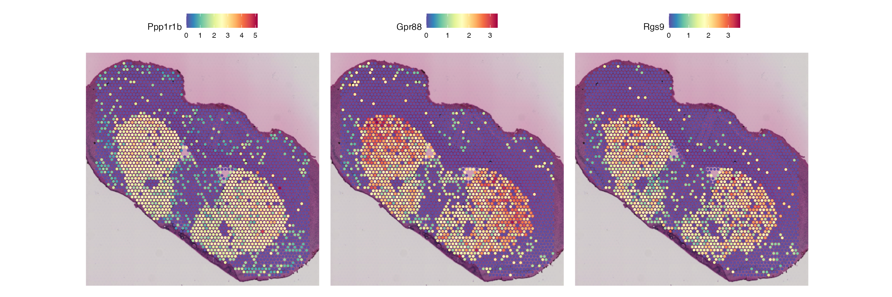
Looking at these results, we can see that our clustering using only genetic information can determine clear morphological brain regions within the Striatum, including the caudoputamen (CP) and nucleus accumbens (ACB). However, clustering using genetic information cannot identify lesioned regions of the Striatum, where the Striatum cells of left hemisphere produce significantly higher levels of Dopamine.
Idents(combined.data) <- "ST_clusters"
DE <- FindAllMarkers(combined.data, only.pos = T)
## prints top 5 genes for cluster 0 == Striatum
head(DE[DE$cluster == 0,] , n =5 )| p_val | avg_log2FC | pct.1 | pct.2 | p_val_adj | cluster | gene | |
|---|---|---|---|---|---|---|---|
| Ppp1r1b | 0 | 2.608029 | 0.958 | 0.342 | 0 | 0 | Ppp1r1b |
| Gpr88 | 0 | 2.781403 | 0.928 | 0.285 | 0 | 0 | Gpr88 |
| Rgs9 | 0 | 2.762431 | 0.884 | 0.232 | 0 | 0 | Rgs9 |
| Pde1b | 0 | 2.363405 | 0.969 | 0.440 | 0 | 0 | Pde1b |
| Penk | 0 | 2.519103 | 0.981 | 0.389 | 0 | 0 | Penk |
Looking at the top 5 most over-expressed genes in cluster 0, we can see some key genes that define the Striatum. These are plot below:
SpatialFeaturePlot(combined.data, features = c("Ppp1r1b", "Gpr88", "Rgs9"), pt.size.factor = 2) 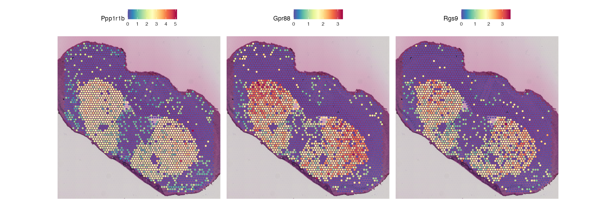
Identified in the original publication, the gene, ‘Pcp4’, was highlighted as differentially expressed between the in-tact vs the lesioned Striatum. Because the gene expression alone cannot differentiate between the lesion vs non-lesioned cells this gene is not observed in the top most differentially expressed genes. We will need to look at the metabolic data to identify this gene.
Cluster SM data
Clustering based on metabolic information will likely reveal different information compared to a transcriptomic approach. SM clustering will reveal more about the activity or functioning of different cell types. Lets see how the clustering differs:
DefaultAssay(combined.data) <- "SPM"
## Run SM clustering
combined.data <- NormalizeData(combined.data, assay = "SPM")
combined.data <- FindVariableFeatures(combined.data, verbose = FALSE)
combined.data <- ScaleData(combined.data, verbose = FALSE)
combined.data <- RunPCA(combined.data, npcs = 30, reduction.name = "spm.pca", verbose = FALSE)
combined.data <- FindNeighbors(combined.data, dims = 1:15, reduction = "spm.pca", verbose = FALSE)
combined.data <- RunUMAP(combined.data, dims = 1:15, reduction = "spm.pca", reduction.name = "spm.umap", verbose = FALSE)
combined.data <- FindClusters(combined.data, resolution = 0.5, cluster.name = "SM_clusters", verbose = FALSE)
DimPlot(combined.data, group.by = "SM_clusters", reduction = "spm.umap", cols = SM_palette) |
SpatialDimPlot(combined.data, group.by = "SM_clusters", pt.size.factor = 2.1, cols = SM_palette) |
SpatialDimPlot(combined.data, group.by = "lesion", pt.size.factor = 2.1)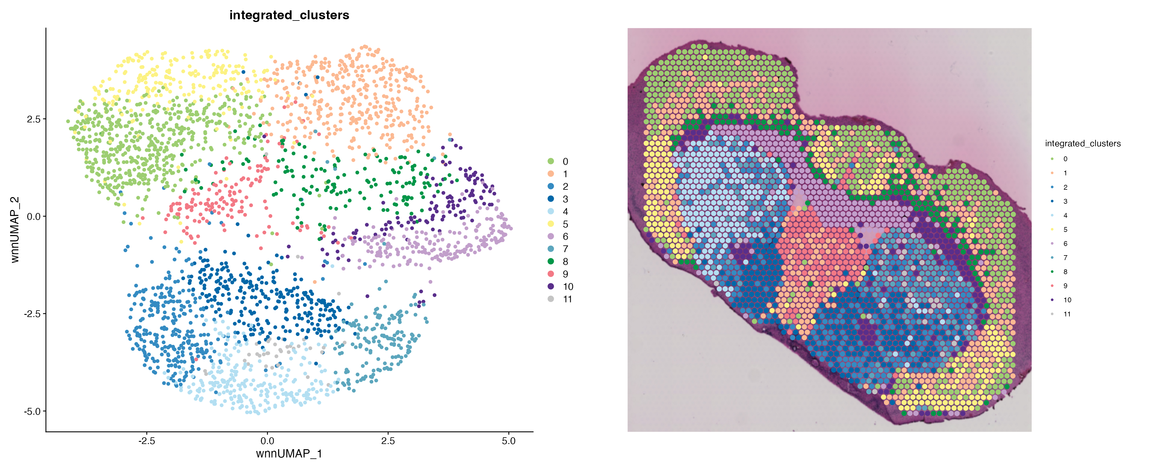
Looking at the clustering results above we can clearly see (cluster 3) defines the cells of the intact Striatum which still produce dopamine. In addition, the spatial distribution of cluster 3 matches the expression pattern of dopamine displayed below:
dopamine_mzs <- SearchAnnotations(combined.data, "Dopamine", assay = "SPM")
combined.data <- BinMetabolites(combined.data, mzs = dopamine_mzs$mz_names, slot = "counts", assay = "SPM", bin_name = "Dopamine")
SpatialFeaturePlot(combined.data, features = "Dopamine", pt.size.factor = 2.1) + theme(legend.position = "right")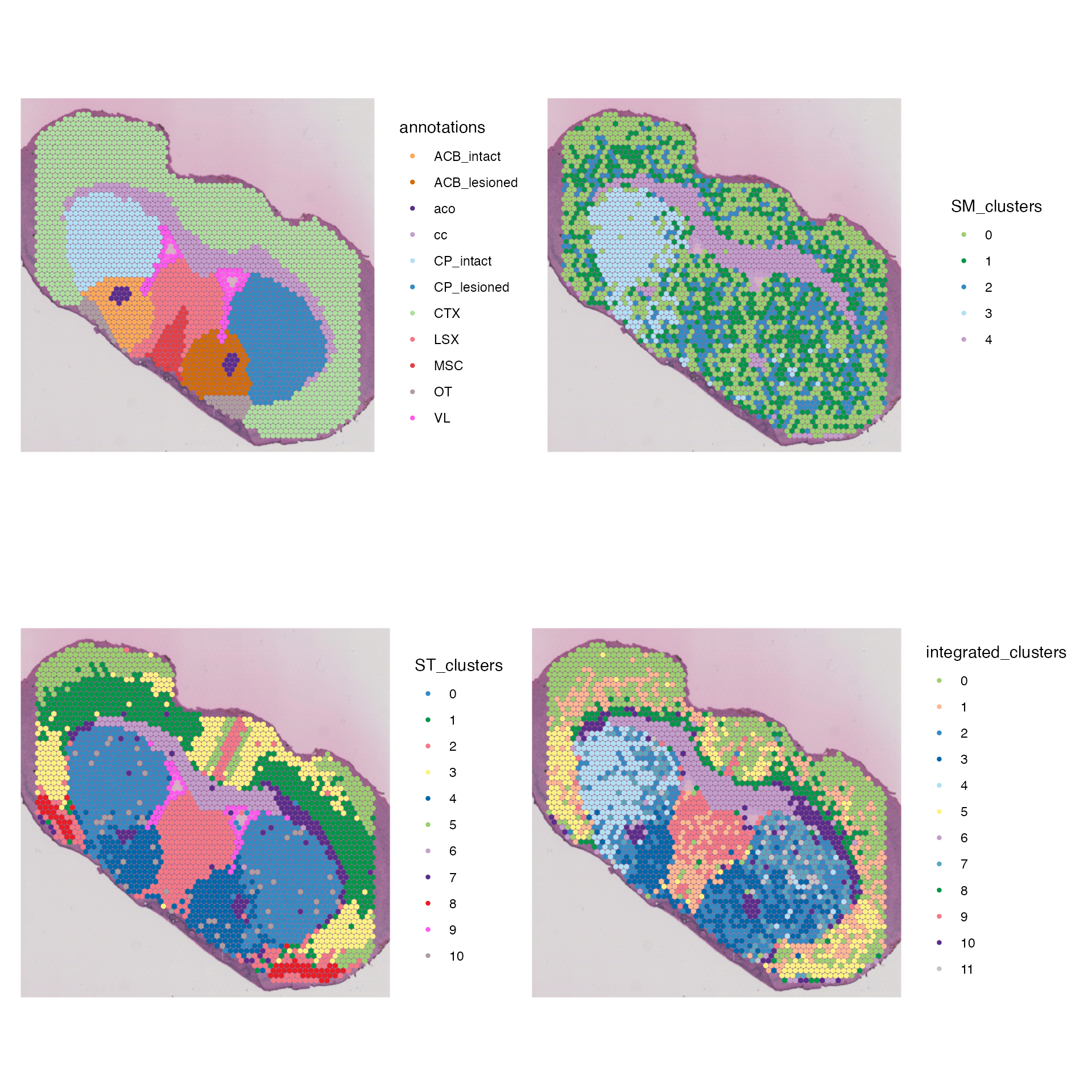
Spatially-Informed Clustering
Seurat based clustering methods provide a fast and robust method for identifying common groups of cells/spots based purely on expression/itensity profiles. However, as seen in the clustering plots above, this method can contain some noise. SpaMTP has implemented a method of clustering based on the python package GraphPCA which uses a spatial nearest-neighbours graph to inform dimensionality reduction and k-means clustering.
Lets perform spatial clsutering on both ST and SM data using
RunSpatialGraphPCA and GetKmeanClusters
below.
## Using GraphPCA to add spatial Infomation
## Run SM clustering
combined.data <- RunSpatialGraphPCA(data = combined.data, n_components = 30, assay = "SPM", platform = "Visium")
combined.data <- GetKmeanClusters(combined.data, cluster.name = "gpca_SPM", clusters = 11)
## Run ST clustering
combined.data <- RunSpatialGraphPCA(data = combined.data, n_components = 30, assay = "SPT", platform = "Visium", reduction_name = "SpatialPCAT", graph_name = "SpatialKNNt")
combined.data <- GetKmeanClusters(combined.data, cluster.name = "gpca_SPT", clusters = 11 ,reduction = "SpatialPCAT")
# Non-Spatial Plots
p1 <- SpatialDimPlot(combined.data, group.by = "ST_clusters", cols = ST_palette, pt.size.factor =2.5, image.alpha = 0.8)
p2 <- SpatialDimPlot(combined.data, group.by = "SM_clusters", cols = SM_palette, pt.size.factor =2.5, image.alpha = 0.8)
#Spatial Plots
p3 <- SpatialDimPlot(combined.data, group.by = "gpca_SPT", cols = spatial_ST_palette, pt.size.factor =2.5, image.alpha = 0.8)
p4 <- SpatialDimPlot(combined.data, group.by = "gpca_SPM", cols = spatial_SM_palette, pt.size.factor =2.5, image.alpha = 0.8)
(p1|p2)/(p3|p4)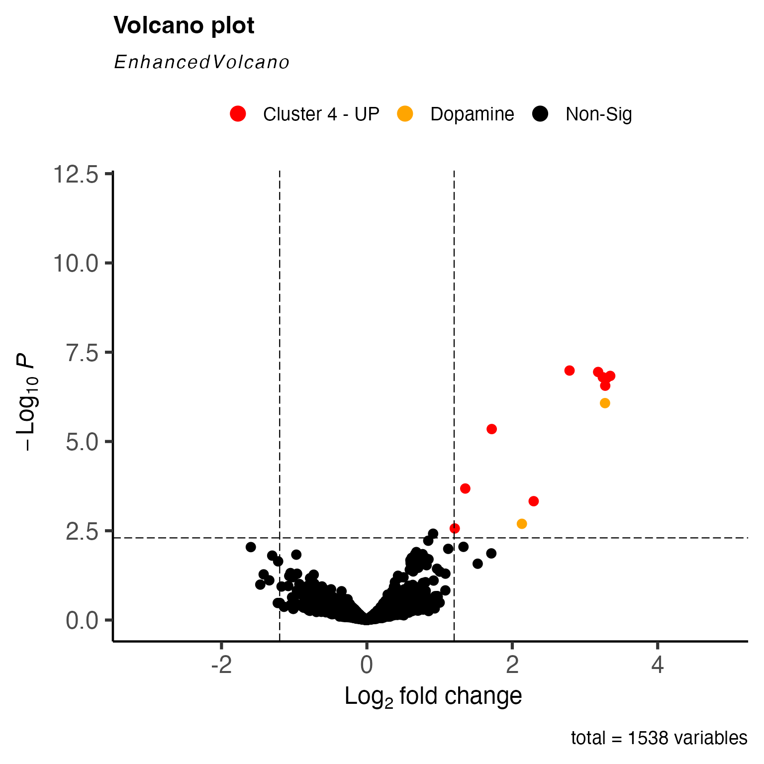 When comparing the results, our GraphPCA-based clustering has much
clearer defined regions with less random noise. These regions also
clearly match biological regions and states such as the lesion and
intact striatum highlighted by cluster 1 (light blue) and cluster 7/8
(dark blue) respectively.
When comparing the results, our GraphPCA-based clustering has much
clearer defined regions with less random noise. These regions also
clearly match biological regions and states such as the lesion and
intact striatum highlighted by cluster 1 (light blue) and cluster 7/8
(dark blue) respectively.
Multi-Modal Integrative Analysis
As explained above, transcriptomic and metabolic data reveal and define different aspects of the tissue. Based on this, multi-modal integration can be used to combine these features into the one analysis. Below we will integrate the spatial transcriptomic and metabolomic data together to get a more refined and detailed clustering result.
The SpaMTP MultiOmicIntegration function allows for automated or manual specification of weights for each modality when generating the integrated clusters. Here we will use pca embeddings generated from our spatially-informed GraphPCA dimentionality reduction and equal modality weights ST = 0.5, SM = 0.5.
integrated.data <- MultiOmicIntegration(combined.data,return.intermediate = T, weight.list = list(0.5,0.5),
reduction.list = list("SpatialPCA", "SpatialPCAT"), dims.list = list(1:30, 1:30))
integrated.data <- RunUMAP(integrated.data, nn.name = "weighted.nn", reduction.name = "wnn.umap", reduction.key = "wnnUMAP_",verbose = FALSE)
integrated.data <- FindClusters(integrated.data, graph.name = "wsnn", algorithm = 3, resolution = 0.6, cluster.name = "integrated_clusters", verbose = FALSE)
DimPlot(integrated.data, group.by = "integrated_clusters", reduction = 'wnn.umap', label = F, cols = intergrated_palette, pt.size = 1.5) |
SpatialDimPlot(integrated.data, group.by = "integrated_clusters", label = F, pt.size.factor = 2.2, cols = intergrated_palette, image.alpha = 1) 
Looking at the results above, we can see the integrative analysis identifies a difference between the lesioned and in-tact striatum cells (cluster 1 and cluster 2 respectively). This difference is also reflected in the UMAP.
We can also compare the difference between ST only, SM only and integrated clustering:
(SpatialDimPlot(integrated.data, group.by = "annotations", pt.size.factor = 2.5, cols = annotation_palette, image.alpha = 0.8)|
SpatialDimPlot(integrated.data, group.by = "gpca_SPM", pt.size.factor = 2.5, cols = spatial_SM_palette, image.alpha = 0.8))/
(SpatialDimPlot(integrated.data, group.by = "gpca_SPT", pt.size.factor = 2.5, cols = spatial_ST_palette, image.alpha = 0.8)|
SpatialDimPlot(integrated.data, group.by = "integrated_clusters", label = F, pt.size.factor = 2.5, cols = intergrated_palette, image.alpha = 0.8))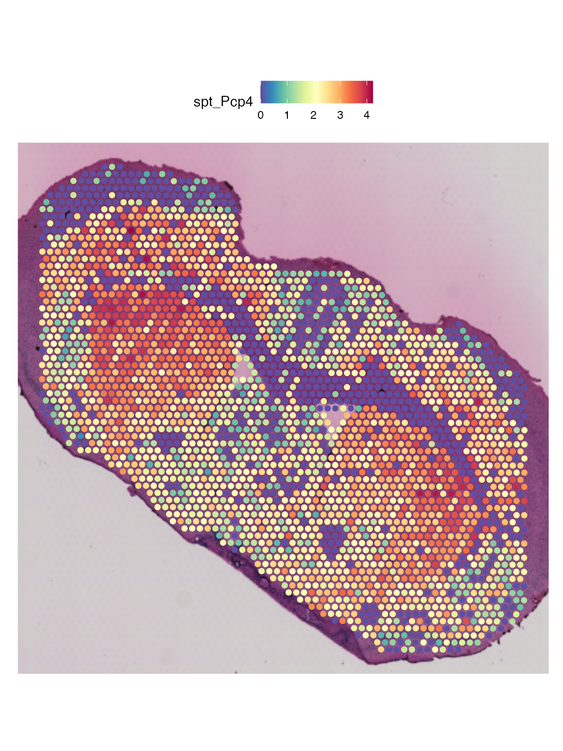
Visually, the integrated clustering highly correlates to the defined annotations. To check this statistically we can quickly calculate an Adjusted Rand Index (ARI) score for each cluster comparted to the annotation ground truth.
# Define clustering columns
clustering_columns <- c("ST_clusters", "SM_clusters", "gpca_SPM", "gpca_SPT", "integrated_clusters")
# Extract metadata
meta <- integrated.data@meta.data
# Ground truth
ground_truth <- as.factor(meta$annotations)
# Compute scores
results <- data.frame(cluster = clustering_columns,ARI = NA)
for (i in seq_along(clustering_columns)) {
pred <- as.factor(meta[[clustering_columns[i]]])
# Ensure matching non-NA values
valid <- !is.na(ground_truth) & !is.na(pred)
results$ARI[i] <- adjustedRandIndex(ground_truth[valid], pred[valid])
}
print(results)| cluster | ARI |
|---|---|
| ST_clusters | 0.3301783 |
| SM_clusters | 0.1653772 |
| gpca_SPM | 0.2292700 |
| gpca_SPT | 0.3450286 |
| integrated_clusters | 0.3871174 |
Based on the results we can see the integrated clustering has the highest ARI score, meaning the clustering is the most similar to the ground truth.
Differential Metabolite and Gene Expression Analysis
Based on this, we can look at which metabolites and genes are differentially expressed between these clusters. First, we will identify which clusters display an up-regulation of dopamine:
# Performs pooling, pseudo-bulking and EdgeR Differential Expression Analysis
cluster_DEMs <- FindAllDEMs(data = integrated.data, ident = "integrated_clusters", n = 3, logFC_threshold = 1.2,
DE_output_dir =NULL, return.individual = FALSE, assay = "SPM",
run_name = "FindAllDEMs", annotation.column = "all_IsomerNames" ) # DE results are returned in a data.framePooling one sample into 3 replicates...
Running edgeR DE Analysis for FindAllDEMs -> with samples [ 3, 1, 2, 4, 7, 5, 6, 9, 0, 8, 10, 11 ]
Starting condition: 3
Starting condition: 1
Starting condition: 2
Starting condition: 4
Starting condition: 7
Starting condition: 5
Starting condition: 6
Starting condition: 9
Starting condition: 0
Starting condition: 8
Starting condition: 10
Starting condition: 11
results <- cluster_DEMs$DEMs[cluster_DEMs$DEMs$cluster == "2",]
metabolites <- c("Dopamine (double derivatized)", "Dopamine (single derivatized)")
### Sets up colouring for significant spots in volcano plot
keyvals <- ifelse(
results$annotations %in% metabolites, "orange", ifelse(
results$logFC < -1.2 & results$P.Value < 50e-4, 'royalblue',
ifelse(results$logFC > 1.2 & results$P.Value < 50e-4, 'red',
'black')))
keyvals[is.na(keyvals)] <- 'black'
names(keyvals)[keyvals == 'red'] <- 'Cluster 2 - UP'
names(keyvals)[keyvals == 'black'] <- 'Non-Sig'
names(keyvals)[keyvals == 'orange'] <- 'Dopamine'
names(keyvals)[keyvals == "royalblue"] <- "Cluster 2 - Down"
### Plots volcano plot with DEM results
volc_plot <- EnhancedVolcano::EnhancedVolcano( results,
selectLab = c(""),
lab = results$annotations,
colCustom = keyvals,
pCutoff = 50e-4,
FCcutoff = 1.2,
pointSize = 3,
colAlpha = 1,
x = 'logFC',
y = 'P.Value',
gridlines.major = FALSE,
gridlines.minor = FALSE)
volc_plot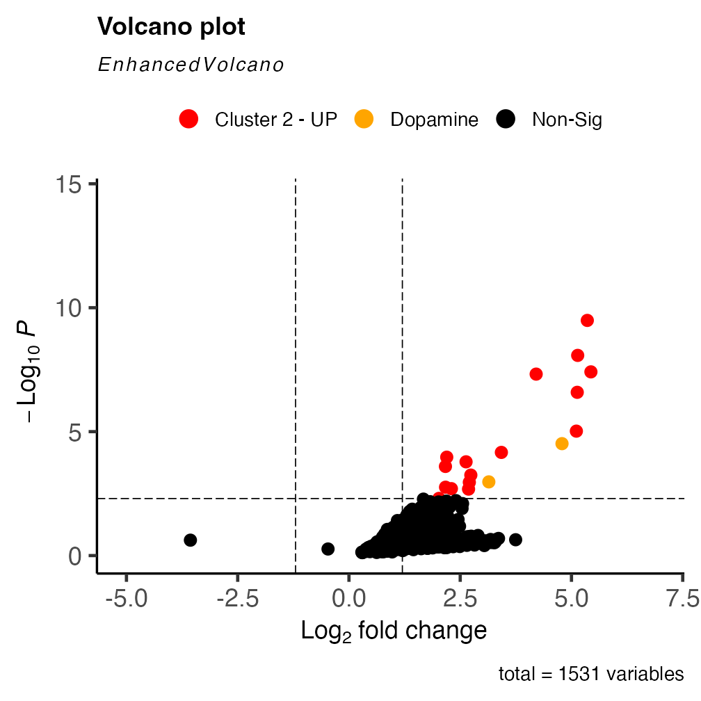
Analysing the DE results, we can see that dopamine (both the single and double FMP10-derivatized) is over expressed in cluster 2.
Now we will look at the gene expression differences between cluster 2 vs all other clusters within the Striatum:
## subset data to only contain the striatum
Idents(integrated.data) <- "integrated_clusters"
striatum <- subset(integrated.data, subset = region == "striatum")
## Find Differentially Expressed Genes
DefaultAssay(striatum) <- "SPT"
striatum_DEGs <- FindAllMarkers(striatum, only.pos = T)
head(striatum_DEGs[striatum_DEGs$cluster == "2",], n = 4)| p_val | avg_log2FC | pct.1 | pct.2 | p_val_adj | cluster | gene | |
|---|---|---|---|---|---|---|---|
| Pcp4 | 0 | 0.6677637 | 0.994 | 0.965 | 0 | 2 | Pcp4 |
| Ppp3ca1 | 0 | 0.3837736 | 1.000 | 0.995 | 0 | 2 | Ppp3ca |
| Camk2n11 | 0 | 0.4997944 | 0.992 | 0.962 | 0 | 2 | Camk2n1 |
| Egr1 | 0 | 0.9936611 | 0.845 | 0.613 | 0 | 2 | Egr1 |
Supporting the findings from the orginal publication, we can see that “Pcp4” is up-regulated in cluster 2 (in-tact striatum cells).
SpatialFeaturePlot(integrated.data, features = "Pcp4", pt.size.factor = 2)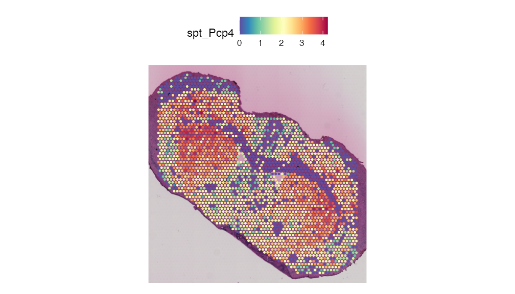
Multi-Omic Data Visualisation
Based on this analysis, we can visualise this gene and metabolite of interest in the same 3D plot (“Pcp4” and “Dopamine”).
Plot3DFeature(combined.data,
features = c("Pcp4", "mz-674.2805"),
assays = c("SPT", "SPM"),
between.layer.height = 10000,
show.image = "slice1",
plot.height = 400,
plot.width = 700,
downscale.image = 2)Multi-Modality Pathway Analysis
In this vignette we will demonstrate two different methods of multi-omic pathway analysis. The first will be a region or cluster based pathway analysis previously described in the Spatial Metabolomics Analysis: Mouse Bladder Vignette. The second method uses the entire expression matrix of each cell.
Cluster-based Pathway Analysis
Now that we have identified there are metabolic and transcriptional differences between the lesioned and intact striatum regions, we can now further assess the activity of each region by performing multi-modal pathway analysis using both genes and metabolites. Another novel feature of SpaMTP is the curated FMP10 annotation database which allows users to run pathway analysis with FMP10 data. Below we will identify pathways based on both genes and metabolites that are significantly altered between striatum regions.
# Generate differential abundance and expression results for integrated clustering
Idents(striatum) <- "integrated_clusters"
deg = FindAllMarkers(striatum, assay = "SPT",only.pos =F)
dem = FindAllMarkers(striatum , assay = "SPM", only.pos =F)
DE.list = list("genes" = deg,"metabolites" = dem)
## Run multi-modal pathway analysis
regpathway = FindRegionalPathways(
striatum,
analyte_types = c("genes", "metabolites"),
SM_slot = "counts", ST_slot = "counts",
ident = "integrated_clusters",
DE.list = DE.list
)
## Select some key pathways to plot
selected_pathways <- c("Epinephrine Action Pathway",
"GABA receptor activation",
"GABA receptor signaling",
"GABAergic synapse",
"Neuroinflammation and glutamatergic signaling",
"Nicotine effect on dopaminergic neurons",
"G alpha (i) signalling events",
"Neuronal System",
"Transmission across Chemical Synapses",
"VEGFA-VEGFR2 signaling",
"Apoptosis")
PlotRegionalPathways(regpathway = regpathway,selected_pathways = selected_pathways)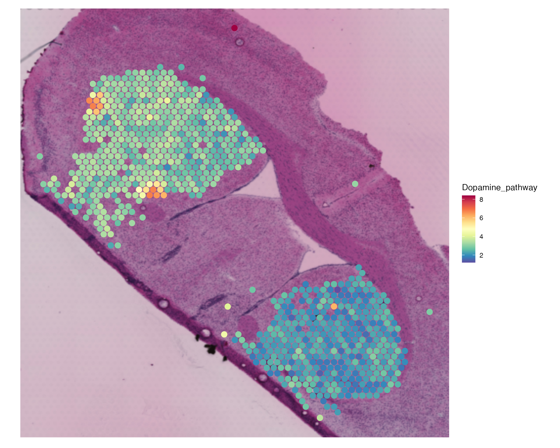
Due to the nature of the FMP10 matrix, there are often only a handful of metabolites annotated meaning some metabolites within various pathwasy are not captured. To resolve this we will run multi-modality pathway analysis using a paired Visium and MALDI DHB-matrix dataset. This data has already been processed with the code hidden below:
DHB Data Processing
### Data was generated and mapped following same steps used above.
### Raw files and metadata for DHB dataset and Visium can be downloaded here. The sample used was V11L12-038_B1: https://figshare.scilifelab.se/articles/dataset/Spatial_Multimodal_analysis_SMA_-_Mass_Spectrometry_Imaging_MSI_/22770161
### Dataset alignment was achieved using the following parameters
###
### Rotation Angle: -0.7
### Move X Axis: 59
### Move Y Axis: -102
### Blue Axis Angle: -45
### Blue Axis Stretch: 1.22
### Red Axis Angle: -45
### Red Axis Stretch: 1.12
### Mirror Y Axis: TRUE
## Using Aligned and Mapped data:
# data(combined.dhb.data)
## Annotate metabolites against databases
#db = rbind(HMDB_db, Chebi_db)
#combined.dhb.data = AnnotateSM(combined.dhb.data,assay = "SPM", db = db, polarity = "positive")
## Normalise ST and SM data
#combined.dhb.data <- NormalizeData(combined.dhb.data, assay = "SPT")
#combined.dhb.data <- NormalizeSMData(combined.dhb.data, assay = "SPM")
## Cluster SM data
#DefaultAssay(combined.dhb.data) <- "SPM"
#combined.dhb.data <- FindVariableFeatures(combined.dhb.data, verbose = FALSE)
# combined.dhb.data <- ScaleData(combined.dhb.data, verbose = FALSE)
# combined.dhb.data <- RunPCA(combined.dhb.data, npcs = 30, reduction.name = "spm.pca", verbose = FALSE)
# combined.dhb.data <- FindNeighbors(combined.dhb.data, dims = 1:30, reduction = "spm.pca", verbose = FALSE)
# combined.dhb.data <- RunUMAP(combined.dhb.data, dims = 1:30, reduction = "spm.pca", reduction.name = "spm.umap", verbose = FALSE)
# combined.dhb.data <- FindClusters(combined.dhb.data, resolution = 0.5, cluster.name = "SM_clusters", verbose = FALSE)
## Isolate the Lesioned vs Intact Striatums
#combined.dhb.data@meta.data <- combined.dhb.data@meta.data %>%
# dplyr::mutate(striatum =
# ifelse((SM_clusters %in% c("0")),
# lesion, "Other"))
## Subset to only lesioned and intact striatum
#striatum.dhb.data <- subset(combined.dhb.data, subset = striatum != "Other")This data object contains the intact and lesioned striatum regions we will be comparing for our multi-modal DHB matrix sample.
striatum_url <- "https://zenodo.org/records/17246900/files/striatum.dhb.data.RDS?download=1"
striatum.dhb.data <- readRDS(url(striatum_url))
SpatialDimPlot(striatum.dhb.data, group.by = "striatum",pt.size.factor = 2)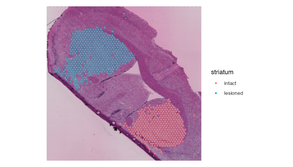
Lets run DE and then find regional pathways
FindRegionalPathways() on our combined data object.
## Run DE analysis for transcriptomics and metabolomics
Idents(striatum.dhb.data) <- "striatum"
deg = FindAllMarkers(striatum.dhb.data , test.use = "wilcox_limma", assay = "SPT",only.pos =F)
dem = FindAllMarkers(striatum.dhb.data , assay = "SPM", only.pos =F)
DE.list = list("genes" = deg,"metabolites" = dem)
## Run multi-modal pathway analysis
regpathway = FindRegionalPathways(
striatum.dhb.data,
analyte_types = c("genes", "metabolites"),
SM_slot = "counts", ST_slot = "counts",
ident = "striatum",
DE.list = DE.list
)We will select some important pathways associated with Parkinson’s disease to plot
selected_pathways = c(
"Dopamine beta-hydroxylase deficiency",
"Tryptophan metabolism",
"Dopamine metabolism",
"sphingolipid metabolism pathway",
"Sphingolipid metabolism: integrated pathway",
"Spermidine and Spermine Biosynthesis",
"Pyruvate metabolism",
"Fatty acid metabolism"
)
PlotRegionalPathways(regpathway = regpathway,selected_pathways = selected_pathways)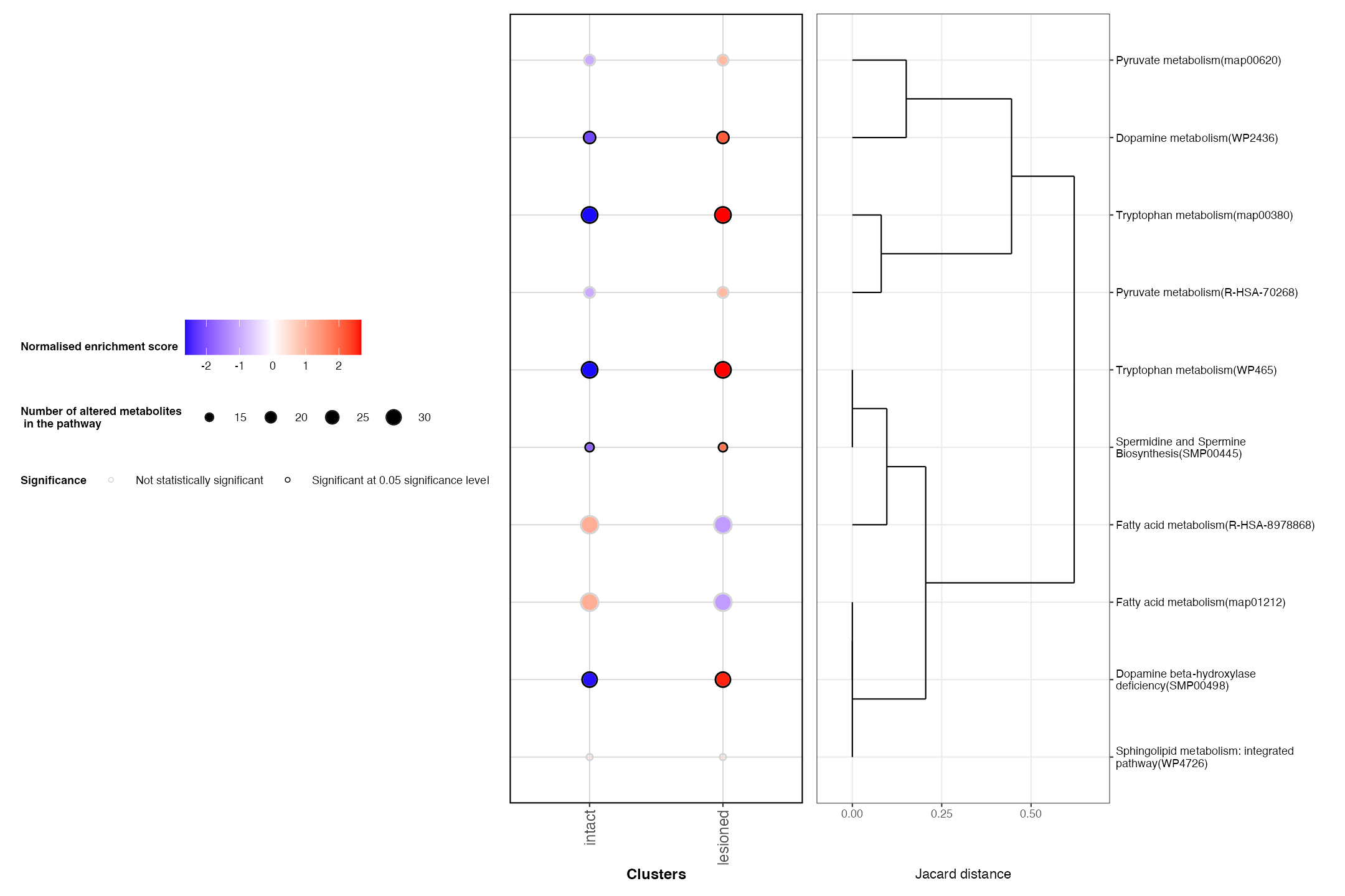
One of the significant pathways associated with the lesioned region was ‘Dopamine beta-hydroxylase deficiency’. We can use SpaMTP’s network plotting function to visualuse the network of this pathway, along with the relative differentially expressed elements that make up the activity of this pathway. Lets have a look:
PathwayNetworkPlots(striatum.dhb.data,ident = "striatum", regpathway = regpathway, DE.list = list("genes" = deg, "metabolites" = dem), selected_pathways = selected_pathways, path = "vignette_data_files/Mouse_Brain/DHB_data")Assuming DE.list[1] contains genes results ....
Assuming DE.list[2] contains metabolites results ....
Query necessary data and establish pathway database
Query db for addtional matching
Constructing DE dataframes....
File successfully written to vignette_data_files/Mouse_Brain/DHB_data/striatum_2024_10_22_12_23_05_AEST.htmlOne key metabolite that was previously not mentioned by the original publication was (R)-S-adenosyl-L-methionine zwitterion. This metabolite has previously been associated with Parkinson’s disease and using SpaMTP, we were able to detect its expression within the lesioned striatum. We will now visualise the expression of this metabolite spatially:
SpatialMZPlot(striatum.dhb.data, mz= 400.14659,plusminus = 0.05, assay = "SPM", pt.size.factor = 2.5, slot = "data") + theme(legend.position = "right")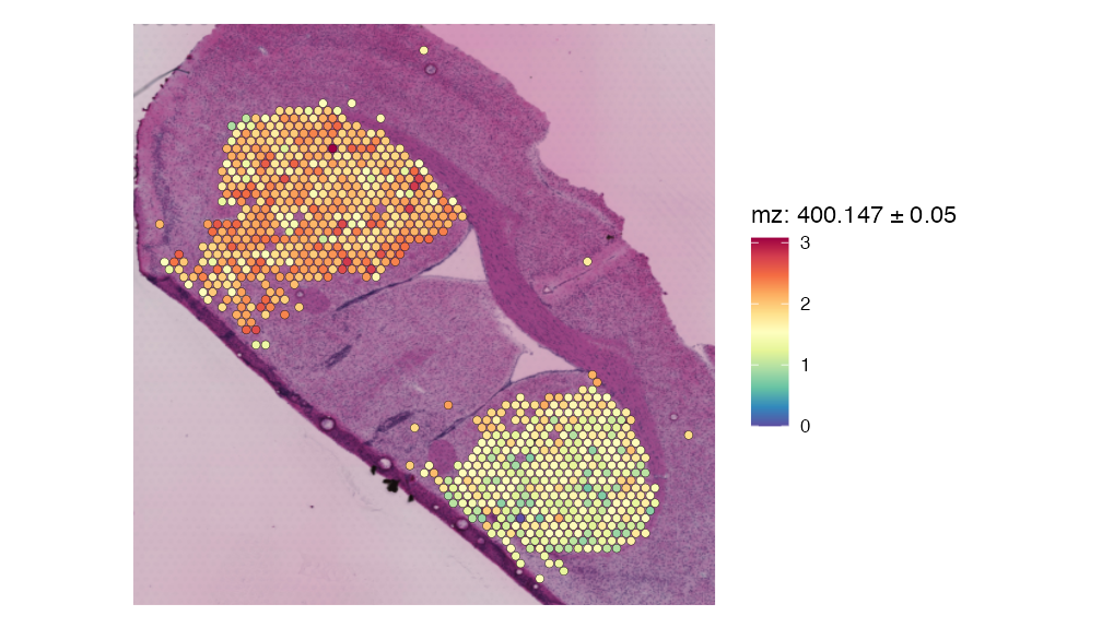
We can see that there is much more expression of this metabolite within the lesioned hemisphere.
Finally, we can combine the expression of each of these metabolites to see the exact region where this pathway is active.
## Get key mz values from network plot
mzs <- c(215.015, 321.08627, 400.14659)
mzs <- unlist(lapply(mzs, function(x){ FindNearestMZ(striatum.dhb.data, target_mz = x, assay = "SPM")}))
striatum.dhb.data <- BinMetabolites(striatum.dhb.data, mzs, slot = "data", bin_name = "Dopamine_pathway", assay = "SPM")
SpatialFeaturePlot(striatum.dhb.data, features = "Dopamine_pathway", pt.size.factor = 2.5) & theme(legend.position = "right") 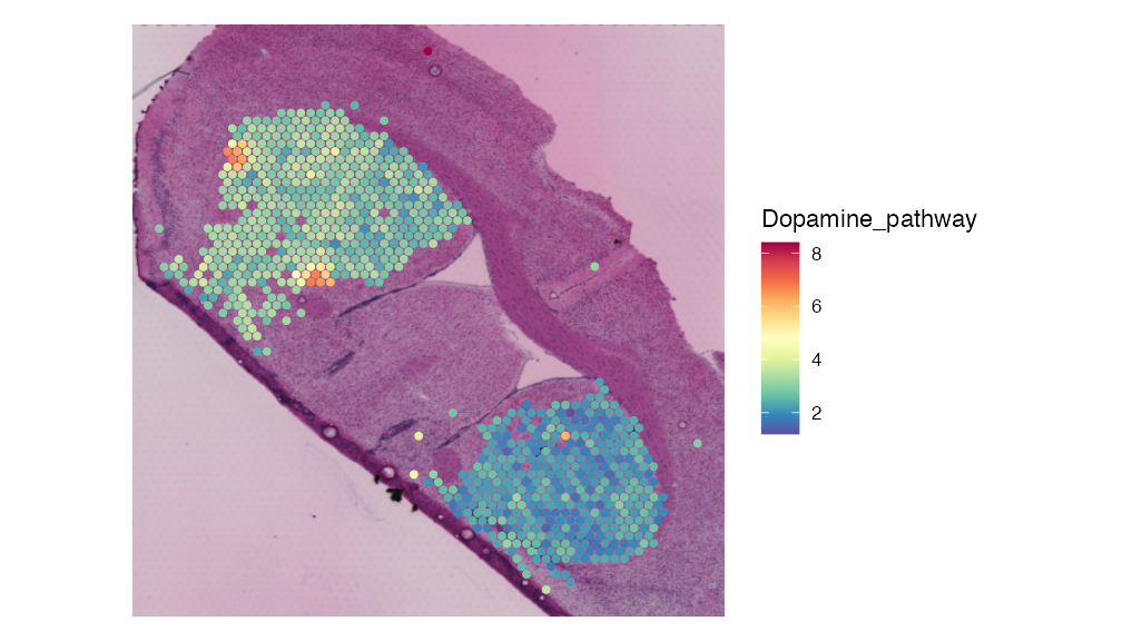
GESECA-Based Pathway Analysis
An alternative method of pathway analysis is using the
RunRAMPgeseca function. This function is based on the gene
set co-regulation analysis tool originally implemented for spatial
transcriptomic analysis. Breifly, this function take in an expression
matrix, where rows and columns correspond to m/z and pixels
respectively, and a list of metabolite pathway sets. This is different
from the FishersPathwayAnalysis and
FindRegionalPathways functions which are based on a
list/ranked list of metabolites, and instead uses intensity values of
all metabolites regardless of wether they are significantly
differentially expressed.
The process involves a few steps:
- Generate a SpaMTP Seurat Object assay with features renaimed to have RAMP_ID names
- Running reverse PCA on the newly generate matrix to calculate a dimentionality reduced expression matrix (E).
- Run
RunRAMPgesecato calculate significantly regulated pathways.
First we will run this approach on our ST and SM data individually. Lets start with ST data:
## Generate pathway assay from ST data only
integrated.data <-CreatePathwayAssay(integrated.data, analyte_type = "genes", assay = "SPT", new_assay = "SPT_pathway")
## Format the new pathway assay correctly for running PCA
DefaultAssay(integrated.data) <- "SPT_pathway"
integrated.data <- NormalizeData(integrated.data)
integrated.data <- ScaleData(integrated.data)
integrated.data <- FindVariableFeatures(integrated.data, nfeatures = 3000)
## Calculate reverse PCA
integrated.data <- RunPCA(integrated.data, assay = "SPT_pathway", verbose = FALSE,
rev.pca = TRUE, reduction.name = "pca.rev.ST",
reduction.key="PCRt_", npcs = 50)
## Extract the feature loadings as our expression matrix
E <- integrated.data@reductions$pca.rev.ST@feature.loadings
## Run geseca-based pathway analysis
ST_results <- RunRAMPgeseca(E, minSize = 3, maxSize = 500, center = FALSE)We can visualise the top 6 most significant pathways:
head(ST_results)| pathway | pctVar | pval | padj | log2err | size |
|---|---|---|---|---|---|
| Transmission across Chemical Synapses | 1.2387703 | 0 | 0 | 1.1239150 | 113 |
| Neuronal System | 1.4227697 | 0 | 0 | 1.1053366 | 170 |
| Glycolysis / Gluconeogenesis | 0.9018126 | 0 | 0 | 1.0864405 | 33 |
| Synaptic vesicle pathway | 0.7357405 | 0 | 0 | 0.9969862 | 25 |
| HIF-1 signaling pathway | 0.8110382 | 0 | 0 | 0.9969862 | 19 |
| Biosynthesis of amino acids | 0.8298095 | 0 | 0 | 0.9436322 | 11 |
Lets plot these:
## Get top 6 pathways
topPathways <- ST_results[, pathway] |> head(6)
## Plot top 6 pathways
plots <- PlotPathwaysSpatially(topPathways, integrated.data, images = c("slice1"), assay = "SPT_pathway", image.alpha = 0, pt.size.factor = 2.5)
## Arrange plots on the same pannel
wrap_plots(plots, ncol = 3)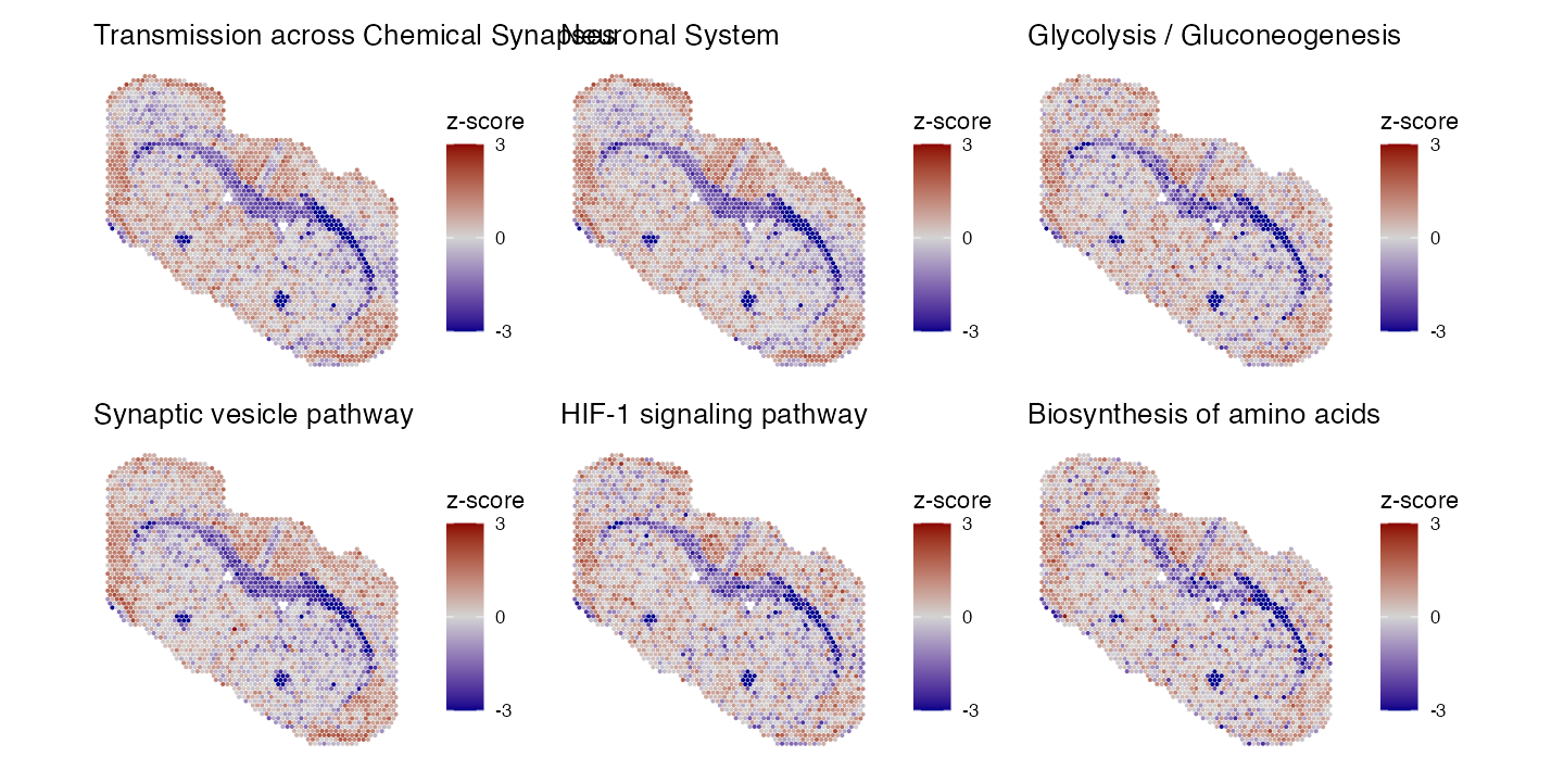
We can see these pathways share a similar expression, with particularly low levels in the corpus callosum. Lets do the same for our SM data:
## Generate pathway assay from SM data only
integrated.data <-CreatePathwayAssay(integrated.data, analyte_type = "metabolites", assay = "SPM", new_assay = "SPM_pathway")
## Format the new pathway assay correctly for running PCA
DefaultAssay(integrated.data) <- "SPM_pathway"
integrated.data <- NormalizeData(integrated.data)
integrated.data <- ScaleData(integrated.data)
integrated.data <- FindVariableFeatures(integrated.data, nfeatures = 3000)
## Calculate reverse PCA
integrated.data <- RunPCA(integrated.data, assay = "SPM_pathway", verbose = FALSE,
rev.pca = TRUE, reduction.name = "pca.rev.SM",
reduction.key="PCRm_", npcs = 50)
## Extract the feature loadings as our expression matrix
E <- integrated.data@reductions$pca.rev.SM@feature.loadings
## Run geseca-based pathway analysis
SM_results <- RunRAMPgeseca(E, minSize = 3, maxSize = 500, center = FALSE)
head(SM_results)| pathway | pctVar | pval | padj | log2err | size |
|---|---|---|---|---|---|
| Prostaglandin and leukotriene metabolism in senescence | 0.3352603 | 0.0e+00 | 0.00e+00 | NA | 5 |
| Quercetin and Nf-kB / AP-1 induced apoptosis | 0.3352603 | 0.0e+00 | 0.00e+00 | NA | 5 |
| Eicosanoid ligand-binding receptors | 0.2682083 | 0.0e+00 | 0.00e+00 | NA | 4 |
| Eicosanoids | 0.2682083 | 0.0e+00 | 0.00e+00 | NA | 4 |
| Prostanoid ligand receptors | 0.2682083 | 0.0e+00 | 0.00e+00 | NA | 4 |
| Arachidonic acid (AA, ARA) oxylipin metabolism | 0.7167236 | 2.3e-06 | 2.24e-05 | 0.6272567 | 16 |
We can see that the top pathways based on our metabolic data are different our transcriptomic analysis. In the case of our Parkinson’s mouse brain dataset, we are interested in pathways related to dopamine. Lets compare the expression of these pathways based on metabolic and transcriptomic data:
## Select pathways of interest
selected_pathways <- c("Parkinson's disease pathway", "Parkinson disease", "Dopamine beta-hydroxylase deficiency", "Dopaminergic synapse","Dopamine metabolism", "Dopamine Activation of Neurological Reward System", "Dopamine Neurotransmitter Release Cycle")
ST_results[ST_results$pathway %in% selected_pathways,]| pathway | pctVar | pval | padj | log2err | size |
|---|---|---|---|---|---|
| Dopamine Neurotransmitter Release Cycle | 0.4868043 | 0.0000000 | 0.0000000 | 0.7881868 | 17 |
| Parkinson disease | 0.2702465 | 0.0000581 | 0.0002762 | 0.5384341 | 7 |
| Dopaminergic synapse | 0.1744391 | 0.0017212 | 0.0030391 | 0.4550599 | 10 |
| Parkinson’s disease pathway | 0.0730078 | 0.3276723 | 0.8720755 | 0.0653834 | 12 |
| Dopamine Activation of Neurological Reward System | 0.0416302 | 0.3546454 | 0.9022491 | 0.0615707 | 3 |
| Dopamine metabolism | 0.0234104 | 0.6013986 | 1.0000000 | 0.0371479 | 3 |
SM_results[SM_results$pathway %in% selected_pathways,]| pathway | pctVar | pval | padj | log2err | size |
|---|---|---|---|---|---|
| Dopamine metabolism | 0.0634961 | 0.4685315 | 0.9786003 | 0.0486034 | 4 |
| Dopamine beta-hydroxylase deficiency | 0.0863300 | 0.5844156 | 0.9786003 | 0.0384787 | 11 |
Only some pathways are significant between the two modalities. We can also spatially visualise these pathways, lets pick 3 to view:
key_pathways <- c("Parkinson disease", "Dopamine beta-hydroxylase deficiency", "Dopamine metabolism")
p1 <- PlotPathwaysSpatially(key_pathways, integrated.data, images = c("slice1"), assay = "SPT_pathway", image.alpha = 0, pt.size.factor = 2.5)
p2 <- PlotPathwaysSpatially(key_pathways, integrated.data, images = c("slice1"), assay = "SPM_pathway", image.alpha = 0, pt.size.factor = 2.5)
wrap_plots(p1, ncol = 3)+plot_annotation(title = "ST Pathways")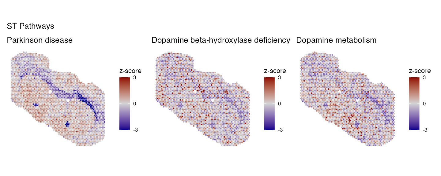
wrap_plots(p2, ncol = 3)+plot_annotation(title = "SM Pathways")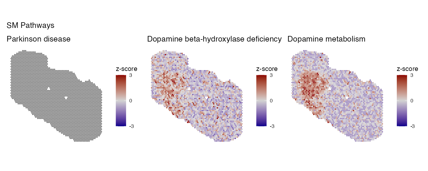
There are clear differences between the two modalities, most likely due to the incomplete feature lists of each pathway when only using one modality. To solve this we can run multi-modal pathway analysis using the data generated above.
## Generate pathway assay from merging SM and ST pathway expression matricies
integrated.data <- CreateMergedModalityAssay(integrated.data, assays.to.merge = c("SPT_pathway","SPM_pathway"))
## Format the new pathway assay correctly for running PCA
DefaultAssay(integrated.data) <- "merged"
VariableFeatures(integrated.data) <- rownames(integrated.data@assays$merged) # To ensure features from both modalities are included
## Calculate reverse PCA
integrated.data <- RunPCA(integrated.data, assay = "merged", verbose = FALSE,
rev.pca = TRUE, reduction.name = "pca.rev.merged",
reduction.key="PCRmerged_", npcs = 50)
## Extract the feature loadings as our expression matrix
E <- integrated.data@reductions$pca.rev.merged@feature.loadings
## Run geseca-based pathway analysis
multiomic_results <- RunRAMPgeseca(E, minSize = 3, maxSize = 500, center = FALSE)
multiomic_results[multiomic_results$pathway %in% selected_pathways,]| pathway | pctVar | pval | padj | log2err | size |
|---|---|---|---|---|---|
| Parkinson disease | 0.1010423 | 0.0000022 | 0.0000184 | 0.6272567 | 31 |
| Dopamine Neurotransmitter Release Cycle | 0.0729224 | 0.0000055 | 0.0000425 | 0.6105269 | 24 |
| Dopaminergic synapse | 0.0303710 | 0.0021274 | 0.0040996 | 0.4317077 | 26 |
| Dopamine beta-hydroxylase deficiency | 0.0249789 | 0.0071759 | 0.0090139 | 0.4070179 | 28 |
| Dopamine metabolism | 0.0167116 | 0.0379620 | 0.7582035 | 0.2311267 | 16 |
| Parkinson’s disease pathway | 0.0105715 | 0.1158841 | 0.7582035 | 0.1262540 | 38 |
| Dopamine Activation of Neurological Reward System | 0.0104370 | 0.1638362 | 0.7582035 | 0.1031975 | 7 |
We can see that all 7 selected pathways associated with dopamine display significantly co-regulation with regions across our sample. Lets now visualise the expression of these pathways spatially:
#key_pathways <- c("Parkinson disease", "Dopamine beta-hydroxylase deficiency", "Dopamine metabolism")
p1 <- PlotPathwaysSpatially(selected_pathways, integrated.data, images = c("slice1"), assay = "merged", image.alpha = 0, pt.size.factor = 2.5)
wrap_plots(p1, ncol = 3)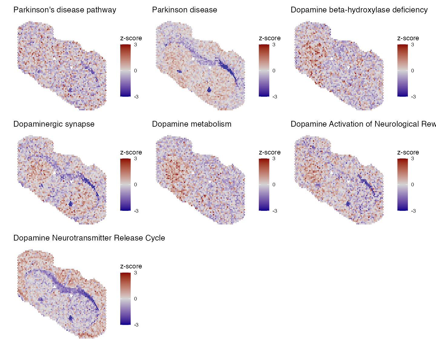
Spatially these pathways show differential expression between the lesioned and intact striatum regions.
## R version 4.4.1 (2024-06-14)
## Platform: aarch64-apple-darwin20
## Running under: macOS 15.5
##
## Matrix products: default
## BLAS: /Library/Frameworks/R.framework/Versions/4.4-arm64/Resources/lib/libRblas.0.dylib
## LAPACK: /Library/Frameworks/R.framework/Versions/4.4-arm64/Resources/lib/libRlapack.dylib; LAPACK version 3.12.0
##
## locale:
## [1] en_US.UTF-8/en_US.UTF-8/en_US.UTF-8/C/en_US.UTF-8/en_US.UTF-8
##
## time zone: Europe/Oslo
## tzcode source: internal
##
## attached base packages:
## [1] stats4 stats graphics grDevices utils datasets methods
## [8] base
##
## other attached packages:
## [1] future_1.67.0 patchwork_1.3.2 mclust_6.1.1
## [4] EnhancedVolcano_1.24.0 ggrepel_0.9.6 ggplot2_4.0.0
## [7] dplyr_1.1.4 Seurat_5.3.0 SeuratObject_5.2.0
## [10] sp_2.2-0 Cardinal_3.8.3 S4Vectors_0.44.0
## [13] ProtGenerics_1.38.0 BiocGenerics_0.52.0 BiocParallel_1.40.2
## [16] SpaMTP_1.1.0
##
## loaded via a namespace (and not attached):
## [1] fs_1.6.6 matrixStats_1.5.0
## [3] spatstat.sparse_3.1-0 bitops_1.0-9
## [5] sf_1.0-21 EBImage_4.48.0
## [7] httr_1.4.7 RColorBrewer_1.1-3
## [9] tools_4.4.1 sctransform_0.4.2
## [11] R6_2.6.1 lazyeval_0.2.2
## [13] uwot_0.2.3 withr_3.0.2
## [15] gridExtra_2.3 progressr_0.16.0
## [17] cli_3.6.5 Biobase_2.66.0
## [19] textshaping_1.0.3 spatstat.explore_3.5-3
## [21] fastDummies_1.7.5 shinyjs_2.1.0
## [23] labeling_0.4.3 sass_0.4.10
## [25] S7_0.2.0 spatstat.data_3.1-8
## [27] proxy_0.4-27 ggridges_0.5.7
## [29] pbapply_1.7-4 pkgdown_2.1.3
## [31] systemfonts_1.2.3 svglite_2.2.1
## [33] scater_1.34.1 parallelly_1.45.1
## [35] CardinalIO_1.4.0 limma_3.62.2
## [37] rstudioapi_0.17.1 FNN_1.1.4.1
## [39] generics_0.1.4 ica_1.0-3
## [41] spatstat.random_3.4-2 crosstalk_1.2.2
## [43] Matrix_1.7-4 ggbeeswarm_0.7.2
## [45] abind_1.4-8 lifecycle_1.0.4
## [47] yaml_2.3.10 edgeR_4.4.2
## [49] SummarizedExperiment_1.36.0 SparseArray_1.6.2
## [51] Rtsne_0.17 grid_4.4.1
## [53] promises_1.3.3 crayon_1.5.3
## [55] miniUI_0.1.2 lattice_0.22-7
## [57] beachmat_2.22.0 cowplot_1.2.0
## [59] zeallot_0.2.0 pillar_1.11.1
## [61] knitr_1.50 fgsea_1.32.4
## [63] GenomicRanges_1.58.0 future.apply_1.20.0
## [65] codetools_0.2-20 fastmatch_1.1-6
## [67] glue_1.8.0 spatstat.univar_3.1-4
## [69] data.table_1.17.8 vctrs_0.6.5
## [71] png_0.1-8 spam_2.11-1
## [73] gtable_0.3.6 cachem_1.1.0
## [75] xfun_0.53 S4Arrays_1.6.0
## [77] mime_0.13 survival_3.8-3
## [79] SingleCellExperiment_1.28.1 units_0.8-7
## [81] statmod_1.5.0 fitdistrplus_1.2-4
## [83] ROCR_1.0-11 nlme_3.1-168
## [85] matter_2.8.0 RcppAnnoy_0.0.22
## [87] GenomeInfoDb_1.42.3 bslib_0.9.0
## [89] irlba_2.3.5.1 vipor_0.4.7
## [91] KernSmooth_2.23-26 DBI_1.2.3
## [93] tidyselect_1.2.1 compiler_4.4.1
## [95] ontologyIndex_2.12 BiocNeighbors_2.0.1
## [97] xml2_1.4.0 desc_1.4.3
## [99] ggdendro_0.2.0 DelayedArray_0.32.0
## [101] plotly_4.11.0 scales_1.4.0
## [103] classInt_0.4-11 lmtest_0.9-40
## [105] tiff_0.1-12 stringr_1.5.2
## [107] digest_0.6.37 goftest_1.2-3
## [109] fftwtools_0.9-11 spatstat.utils_3.2-0
## [111] rmarkdown_2.29 XVector_0.46.0
## [113] htmltools_0.5.8.1 pkgconfig_2.0.3
## [115] jpeg_0.1-11 MatrixGenerics_1.18.1
## [117] fastmap_1.2.0 rlang_1.1.6
## [119] htmlwidgets_1.6.4 UCSC.utils_1.2.0
## [121] shiny_1.11.1 farver_2.1.2
## [123] jquerylib_0.1.4 zoo_1.8-14
## [125] jsonlite_2.0.0 BiocSingular_1.22.0
## [127] RCurl_1.98-1.17 magrittr_2.0.4
## [129] kableExtra_1.4.0 scuttle_1.16.0
## [131] GenomeInfoDbData_1.2.13 dotCall64_1.2
## [133] Rcpp_1.1.0 ggnewscale_0.5.2
## [135] viridis_0.6.5 reticulate_1.43.0
## [137] stringi_1.8.7 zlibbioc_1.52.0
## [139] MASS_7.3-65 plyr_1.8.9
## [141] parallel_4.4.1 listenv_0.9.1
## [143] deldir_2.0-4 splines_4.4.1
## [145] tensor_1.5.1 locfit_1.5-9.12
## [147] igraph_2.1.4 spatstat.geom_3.6-0
## [149] RcppHNSW_0.6.0 reshape2_1.4.4
## [151] ScaledMatrix_1.14.0 evaluate_1.0.5
## [153] httpuv_1.6.16 RANN_2.6.2
## [155] tidyr_1.3.1 purrr_1.1.0
## [157] polyclip_1.10-7 scattermore_1.2
## [159] rsvd_1.0.5 xtable_1.8-4
## [161] e1071_1.7-16 RSpectra_0.16-2
## [163] later_1.4.4 viridisLite_0.4.2
## [165] class_7.3-23 ragg_1.5.0
## [167] tibble_3.3.0 beeswarm_0.4.0
## [169] IRanges_2.40.1 cluster_2.1.8.1
## [171] globals_0.18.0