SpaMTP: Spatial Metabolomics Analysis
Source:vignettes/Mouse_Urinary_Bladder.Rmd
Mouse_Urinary_Bladder.RmdAnalsysing Spatial Metabolomic Data with SpaMTP
This tutorial highlights the utility of SpaMTP for analysing pixel level or single-cell resolution spatial metabolomics (SM) data. Note: This tutorial has been updated for compatibility with Cardinal V3.8.
Using SpaMTP we will highlight:
- Loading Spatial Metabolomic (SM) Data
- Using Cardinal tools - Tissue Segmentation using SSC
- Automated Metabolite Annotation of m/z Masses
- Simplifying Lipid Nomenclature into Lipid Categories and Classes
- Differential Expression Analysis of Annotated Metabolites
- Metabolite Expression Visualisation
- Pathway Analysis
- Re-Clustering using PCA and Seurat
- Finding Spatially Correlated Metabolites
Author: Andrew Causer
Install and Import R Libraries
First we need to import the required libraries for this analysis.
## Install SpaMTP if not previously installed
if (!require("SpaMTP"))
devtools::install_github("GenomicsMachineLearning/SpaMTP")
#General Libraries
library(SpaMTP)
library(Cardinal)
library(Seurat)
library(dplyr)
#For plotting + DE plots
library(ggplot2)
library(EnhancedVolcano)
library(viridis)Load SM Data using SpaMTP
There are three main ways to load data with SpaMTP. To demonstrate each we will use three different public datasets which you can download or load directly from SpaMTP zenodo page.
1. Converting From a Cardinal Object
The first method is to convert a already loaded Cardinal object directly to a SpaMTP object. This will allow users to analyse any pre-existing cardinal dataset using SpaMTP, and also use pre-processing tools implemented by both packages. To demonstrate this we will load, process and convert the ‘PIGII_206’ pig fetus dataset.
# Load directly from file
#pig206 <- readRDS("./Documents/pig206.RDS")
# Load directly from URL
pig206_url <- "https://zenodo.org/records/17246555/files/pig206.RDS?download=1"
pig206 <- readRDS(file = url(pig206_url))
pig206## MSImagingExperiment with 10200 features and 4959 spectra
## spectraData(1): intensity
## featureData(1): mz
## pixelData(3): x, y, run
## coord(2): x = 10...120, y = 1...66
## runNames(1): PIGII_206
## mass range: 150.0833 to 1000.0000
## centroided: FALSEThis is an unprocessed cardinal object containing 4,959 spectra with 10,200 m/z values ranging between 150 to 1000 m/z. This object can then be processed following Cardinal’s vignette.
pig206 <- summarizeFeatures(pig206, c(Mean="mean"))
pig206_peaks <- pig206 |>
normalize(method="tic") |>
peakProcess(SNR=3, sampleSize=0.1,
tolerance=0.5, units="mz")
pig206_peaks## MSImagingExperiment with 687 features and 4959 spectra
## spectraData(1): intensity
## featureData(3): mz, count, freq
## pixelData(3): x, y, run
## coord(2): x = 10...120, y = 1...66
## runNames(1): PIGII_206
## metadata(1): processing_20260120213413
## mass range: 150.2917 to 999.8333
## centroided: TRUEFollowing our processing steps the cleaned dataset contains 687 peaks. Using Cardinal we can visualise one of these peaks (m/z 537) below which is abundant in the pig liver.
image(pig206_peaks, mz=537.08)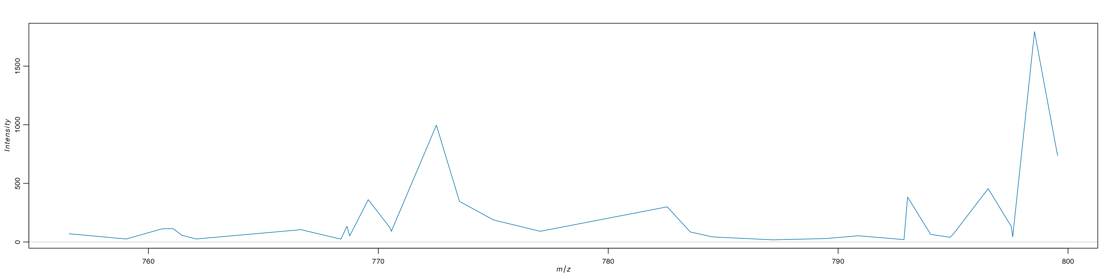
In addition to pre-processing methods, we can also run additional analyses such as Cardinal’s tissue segmentation with spatial shrunken centroids (ssc).
Following the Cardinal’s vignette, we will use the same values for:
- Spatial neighborhood radius = 2
- Maximum number of segments/clusters = 8
- Sparsity thresholding parameter = 2,4,8,16,32,64
set.seed(1)
pig206_ssc <- spatialShrunkenCentroids(pig206_peaks,
weights="adaptive", r=2, k=8, s=2^(1:6))
col_palette = list("1" = "#5aa14f",
"2" = "#4f79a6",
"3" = "#e2585a",
"4" = "#76b8b3",
"5" = "#ebc948",
"6" = "#f18e29")
image(pig206_ssc, i=5,type="class",col= unlist(unname(col_palette)))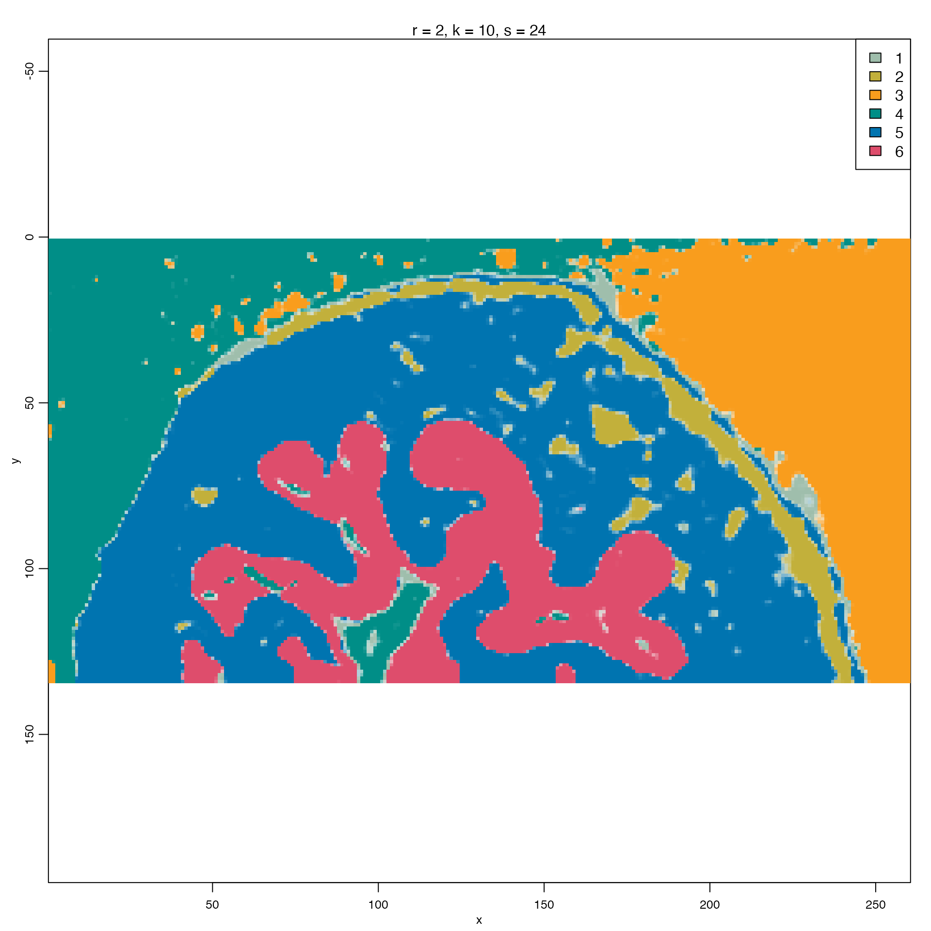
From this we can see areas such as the liver, heart, and brain distinguished as segments 4, 1, and 5 respectively, as presented in the original Cardinal vignette.
Although the majority of functions within the SpaMTP package are used
as wrappers for analysing and modifying Seurat objects, there are a few
functions that are designed to assist in SM analysis in Cardinal. The
function below is one, which allows you to add the SCC results back to a
spectral Cardinal Object, stored in the pixelData slot.
pig206_peaks <- add_ssc_annotation(pig206_peaks, pig206_ssc, resolution = "r=2,k=8,s=32")
pig206_peaks## MSImagingExperiment with 687 features and 4959 spectra
## spectraData(1): intensity
## featureData(3): mz, count, freq
## pixelData(4): x, y, run, ssc
## coord(2): x = 10...120, y = 1...66
## runNames(1): PIGII_206
## metadata(1): processing_20260120213413
## mass range: 150.2917 to 999.8333
## centroided: TRUEOnce finished with the analysis using Cardinal we can use
the SpaMTP function CardinalToSeurat to generate a
SpaMTP object from the processed data.
pig206_spamtp <- CardinalToSeurat(pig206_peaks)
pig206_spamtp## An object of class Seurat
## 687 features across 4959 samples within 1 assay
## Active assay: Spatial (687 features, 0 variable features)
## 1 layer present: counts
## 1 spatial field of view present: fovWe can see like the Cardinal object, the converted SpaMTP object also contains 687 peaks and 4,959 pixels. Furthermore, our ssc results are stored in our SpaMTP object metadata.
head(pig206_spamtp@meta.data, n = 5)| orig.ident | nCount_Spatial | nFeature_Spatial | x | y | run | ssc | |
|---|---|---|---|---|---|---|---|
| 72_1 | SeuratProject | 2010.586 | 599 | 72 | 1 | PIGII_206 | 6 |
| 73_1 | SeuratProject | 2016.971 | 597 | 73 | 1 | PIGII_206 | 3 |
| 74_1 | SeuratProject | 2012.432 | 612 | 74 | 1 | PIGII_206 | 3 |
| 75_1 | SeuratProject | 1996.075 | 597 | 75 | 1 | PIGII_206 | 3 |
| 76_1 | SeuratProject | 2008.766 | 605 | 76 | 1 | PIGII_206 | 3 |
Lets also generate some plots to compare:
ImageMZPlot(pig206_spamtp, mzs = 537.106, size = 2.2, dark.background = F) + scale_x_reverse()+coord_flip()+scale_fill_gradientn(colours = viridis(10))+ ggtitle("SpaMTP")
image(pig206_ssc, i=5,type="class",col= unlist(unname(col_palette)))
title("Cardinal", outer = TRUE)
ImageDimPlot(pig206_spamtp, group.by = "ssc", size = 2.2, dark.background = F, cols = col_palette) + scale_x_reverse()+coord_flip() + ggtitle("SpaMTP")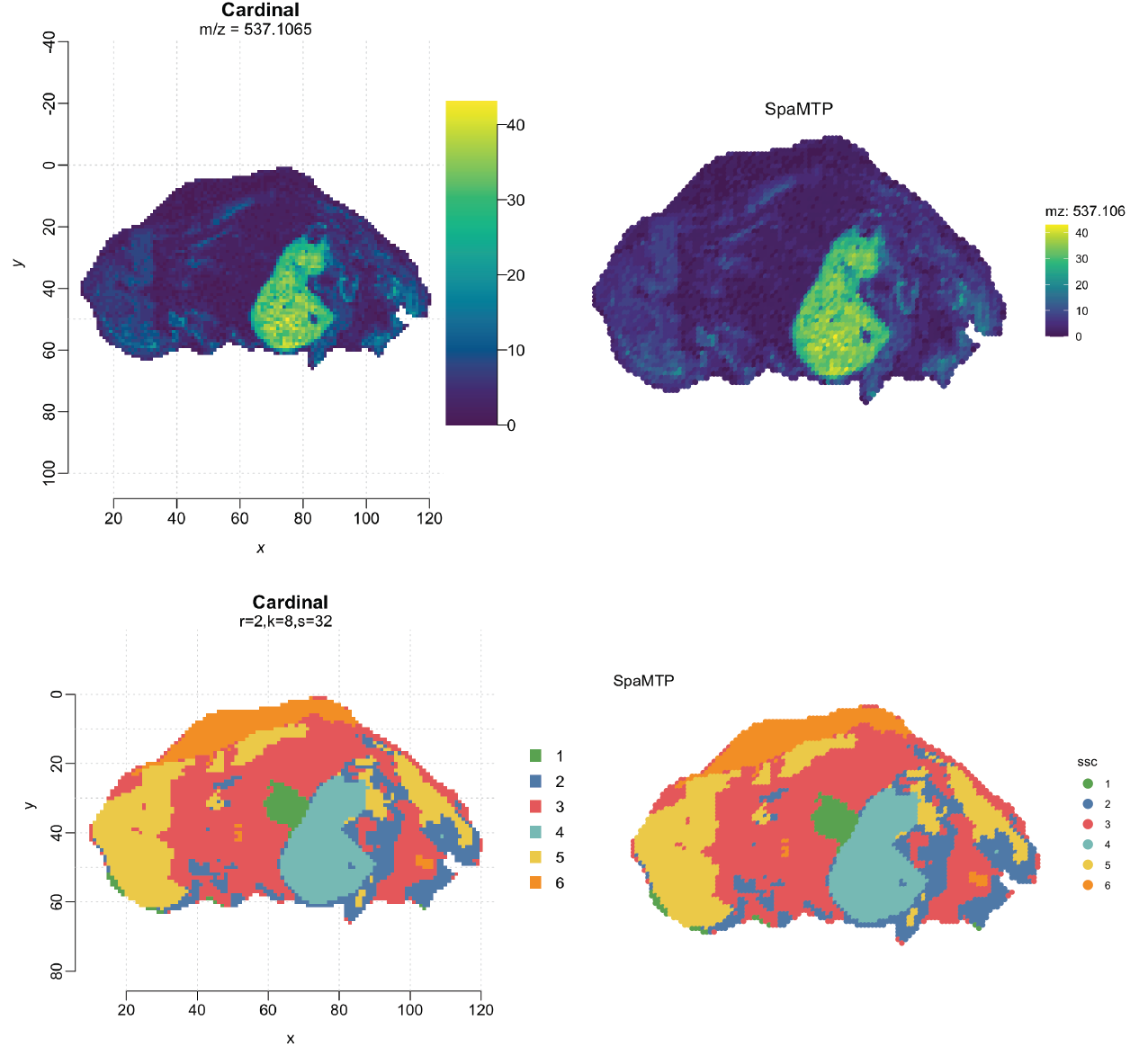
We can see the feature and ssc segment plots match between SpaMTP and Cardinal objects.
2. Load Data Directly
SpaMTP also provides a function for loading data directly
from .ibd and .imzML files. This LoadSM SpaMTP
function is a wrapper on Cardinal’s readImzML() function. For
more information on how this function works, and the relative inputs it
accepts please head to Cardinal’s
documentation page. This function also has capabilities for
splitting data containing multiple runs, into individual SpaMTP
data FOV’s. Below we will use the Human
Renal Cell Carcinoma (RCC) public dataset to demonstrate this.
The corresponding .imzML files can be downloaded directly from SpaMTP zenodo page.
rcc_spamtp## An object of class Seurat
## 10200 features across 16000 samples within 1 assay
## Active assay: Spatial (10200 features, 0 variable features)
## 1 layer present: counts
## 8 spatial fields of view present: fov.1 fov.2 fov.3 fov.4 fov.5 fov.6 fov.7 fov.8This dataset contains 10,200 m/z-values across 8 different runs which are split into individual FOV’s. Each run contains a cancer and normal sample which have been loaded in the metadata. Lets visualise each run in one plot:
ImageDimPlot(rcc_spamtp, group.by = "diagnosis", dark.background = F, fov = names(rcc_spamtp@images), size = 2,
cols = c("red", "blue"),na.value= "white")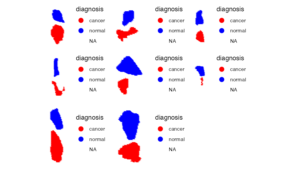
3. Load Intensity Matrix files
The final method of loading SM data into a SpaMTP object is
through an intensity matrix stored in a .csv file. This is
different to .ibd and .imzML files that were used above, the layout of
this dataset is demonstrated below:
| x | y | mz_1 | mz_2 | mz_3 | … | mz_n |
|---|---|---|---|---|---|---|
| 0 | 1 | 0 | 0 | 11 | … | 0 |
| 0 | 2 | 0 | 0 | 0 | … | 0 |
| 0 | 3 | 15 | 0 | 0 | … | 32 |
| 0 | 4 | 20 | 0 | 0 | … | 32 |
| 0 | 5 | 0 | 20 | 0 | … | 0 |
To demonstrate this we will use a public mouse bladder SM data first published by Römpp et al.(2010), and used in the Cardinal V3 article.
NOTE: The data used below is processed data from Cardinal’s V3 Vignette (2023). The raw data is from, “Histology by Mass Spectrometry: Label-Free Tissue Characterization Obtained from High-Accuracy Bioanalytical Imaging”, and can be downloaded from Project PXD001283.
This dataset will be used for the remainder of the tutorial.
# Load directly from file
#bladder <- ReadSM_mtx("./Documents/bladder_csv.csv", mz.prefix = "mz-", feature.start.column = 2)
# Load directly from URL
bladder_url <- "https://zenodo.org/records/17246684/files/bladder_csv.csv?download=1"
bladder <- ReadSM_mtx(mtx.file = bladder_url, mz.prefix = "mz-", feature.start.column = 2)
bladder## An object of class Seurat
## 305 features across 34840 samples within 1 assay
## Active assay: Spatial (305 features, 0 variable features)
## 1 layer present: counts
## 1 spatial field of view present: fovBecause SpaMTP is built on a Seurat Object, we can use useful pre-established Seurat and ggplot2 functions to plot the spatial distribution of the total number of features (m/z’s) present per pixel.
ImageFeaturePlot(bladder, features = "nFeature_Spatial", size = 1) + coord_flip() + scale_x_reverse()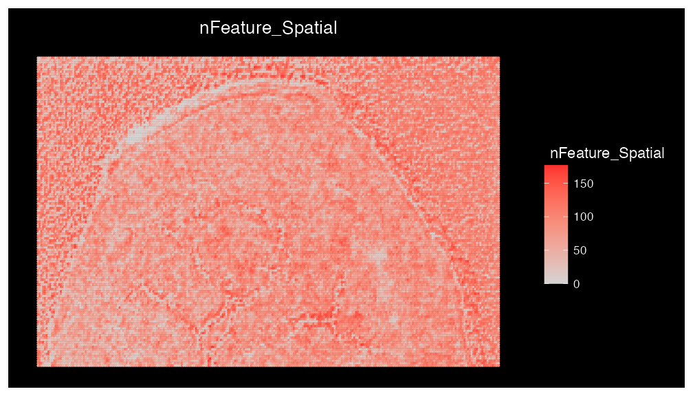
In addition we can also add metadata such as tissue segmentation results from ssc. These segments were generated following parameters specified in Cardinal’s V3 Vignette (2023), with ‘r= 2, k=10, s=24’ using ‘gausian’ weights.
metadata_url <- "https://zenodo.org/records/17246684/files/bladder_metadata.csv?download=1"
bladder_metadata <- read.csv(url(metadata_url), row.names = 1)
head(bladder_metadata, n = 5)| sample | ssc | |
|---|---|---|
| 1_1 | mouse-bladder-peaks | 4 |
| 2_1 | mouse-bladder-peaks | 4 |
| 3_1 | mouse-bladder-peaks | 4 |
| 4_1 | mouse-bladder-peaks | 4 |
| 5_1 | mouse-bladder-peaks | 4 |
bladder@meta.data[colnames(bladder_metadata)]<- bladder_metadata
bladder$ssc <- factor(bladder$ssc) # Required format for some Seurat functionsLets visualise the ssc segmentations added:
col_palette = list("1" = "#9FBEAC",
"2" = "#C2B03B",
"3" = "#F99D1D",
"4" = "#008E87",
"5" = "#0074B0",
"6" = "#DE4D6C",
"7" = "#F99D1D",
"8" = "#DE4D6C",
"9" = "#BF212E")
ImageDimPlot(bladder, group.by = "ssc", cols = col_palette, dark.background = F, size = 2)+ coord_flip() + scale_x_reverse()## Coordinate system already present.
## ℹ Adding new coordinate system, which will replace the existing one.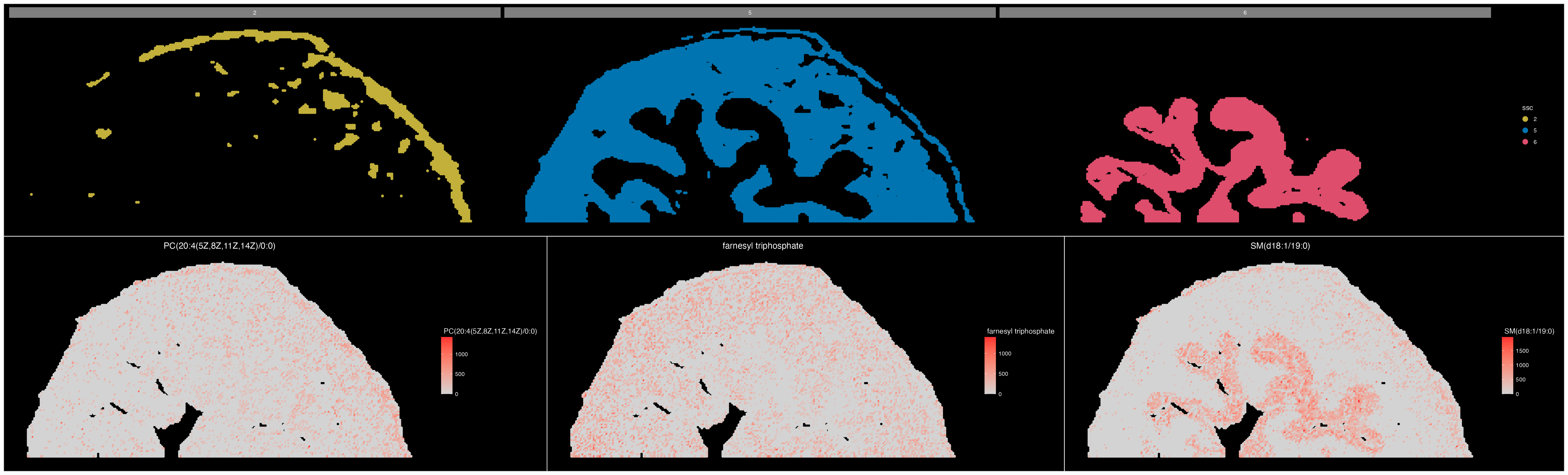
We can see that our segmentation plot matches Cardinal’s previously published results. Published in the original paper by Römpp et al.(2010) we will visualise three m/z values that define organ structures within the urinary bladder.
ImageMZPlot(bladder, mzs = c(770.5104, 770.56, 741.5307), size = 1.5) & coord_flip() & scale_x_reverse()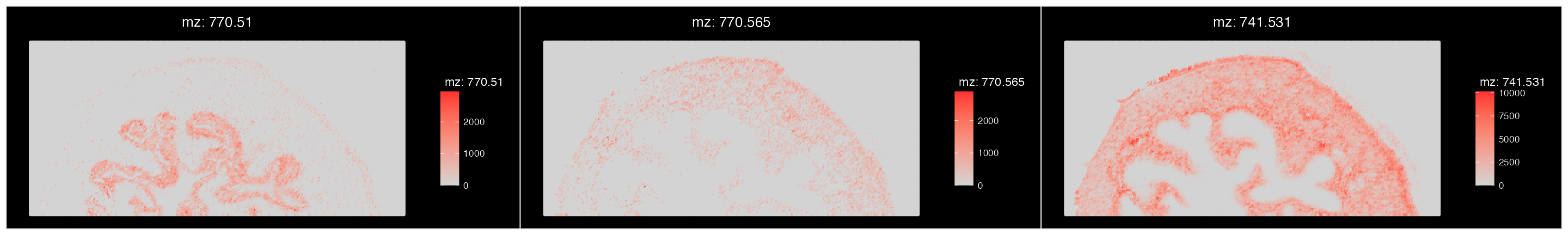
Based on the plots above, there are a few clusters that are associated with regions outside the tissue. It is clear that cluster 3 and 4 are outside the tissue and can therefore be removed.
However, to ensure our dataset is clean of technical noise before we begin downstream analyses we can perform some further data processing and QC.
Sample Pre-Processing and Quality Control
Pre-processing and quality control (QC) are import steps in any pipeline and should be performed prior to any downstream analysis. For spatial metabolic data, there are various packages which have robust functions and applications for removing technical noise from a SM dataset, these include Cardinal and SCILS-LAB as previously described. SpaMTP also provides general pre-processing functions such as data normalisation, scaling and filtering.
Although our data may be normalised and filtered, it still may contains some pixels which are outside the tissue region (cluster 1). To ensure we remove this technical noise we can visualise some QC metrics using SpaMTP.
First we will look at the total number of features and total intensity per pixel between our segments:
VlnPlot(ROI, features = c("nCount_Spatial", "nFeature_Spatial"),group.by = "ssc",cols = col_palette)+ theme_minimal()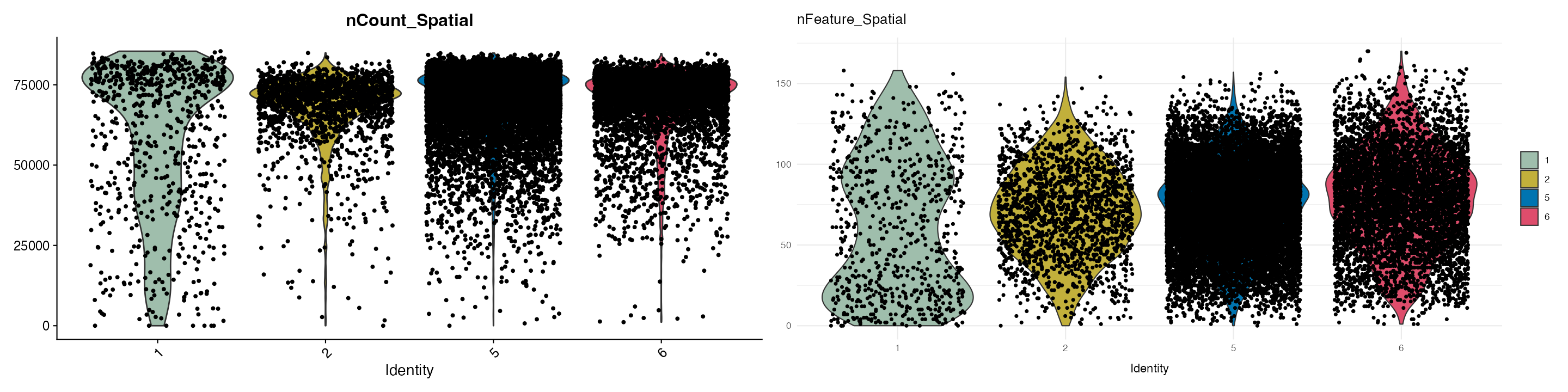
Based on this we can see cluster 1 follows a different distribution compared to the other clusters and is also likely outside the tissue regions. Lets also remove this cluster.
ROI <- subset(ROI, subset = ssc == 1, invert = T)Another metric to assess is the relative intensity values of each m/z across a sample. It is likely a sign of technical noise in cases where some m/z values present with excessively large intensities in comparison to the rest of the dataset. We can visualise this by comparing our raw data to our normalised and filtered dataset.
These plots display the intensity of each m/z summed across all pixels per group. Based on this, the majority of m/z values in our processed data display intensities within a similar distribution, across each cluster, suggesting that there are no outlying m/z values. The unprocessed raw data can be seen to contain some m/z values with excessively large intensities which have been removed through processing.
Using this function we can also look at the distribution of specific features across groups by providing a feature name. Lets try and visualise the total intensity of “mz-740.471557617188” across each cluster using the box.plot function:
MZBoxPlot(seurat.obj = ROI,group.by = "ssc", mzs = "mz-740.471557617188", log.data = TRUE, show.points = F, top.cutoff = 0.05,bottom.cutoff = 0.05,cols = col_palette) 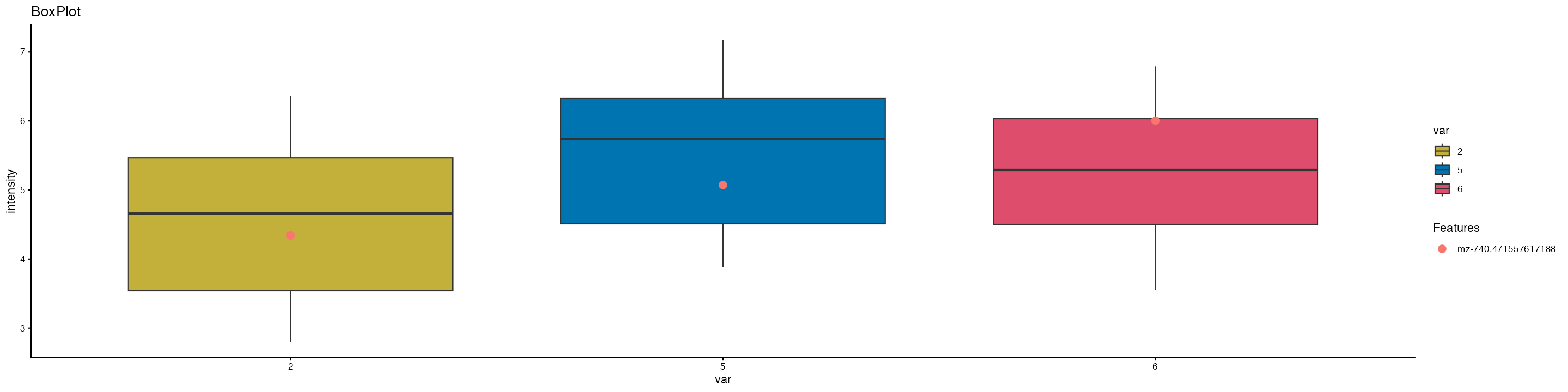
Based on this we can see that the “mz = 740.471557617188” is expressed in all clusters and is highest in cluster 6.
Similar to before we can interchangeably convert our data between
SpaMTP and Cardinal objects, meaning pre-processing or
analysis tools from either package can be used at any point during the
analysis pipeline. We will demonstrate how to use the
ConvertSeuratToCardinal function later in this tutorial. As
we have demonstrated our data is of good quality we can continue our
analysis.
Metabolite Annotation of m/z Masses
One of the major steps in the analysis of metabolomics is the identification/annotation of m/z masses to their relative common metabolite name. There are various public websites that can be used to run this, however, they are often complicated and do not take in an R object or annotate them directly.
SpaMTP has a user-friendly function that assigns possible annotations to each m/z value based on a few variables:
- db: Database to query the m/z masses against -> options are = “HMDB”, “LipidMaps”, “GNPS” or “ChEBI”
- polarity: Polarity mode the experiment was run in -> either “positive” or “negative”
- adducts: Specify different adduct ions that are likely formed or lost during the mass spectrometry imaging.
bladder_annotated <- AnnotateSM(bladder, db = Lipidmaps_db, ppm_error = 15, adducts = "M+K", polarity = "positive")Filtering 'Lipidmaps_db' database by M+K adduct/s
Searching database against input m/z's to return annotaiton results
Adding annotations to Seurat Object ....
Returning Seurat object that include ONLY SUCCESSFULLY ANNOTATED m/z features
bladder_annotated## An object of class Seurat
## 79 features across 34840 samples within 1 assay
## Active assay: Spatial (79 features, 0 variable features)
## 1 layer present: counts
## 1 spatial field of view present: fovFollowing annotation with the LIPID_MAPS database, there are 79 m/z masses that were successfully annotated!
These annotations are stored in the feature meta.data slot within our SpaMTP Object, lets take a look:
head(bladder_annotated[["Spatial"]]@meta.data, n = 3)| raw_mz | mz_names | observed_mz | all_IsomerNames | all_Isomers | all_Isomers_IDs | all_Adducts | all_Formulas | all_Errors | |
|---|---|---|---|---|---|---|---|---|---|
| 16 | 426.9289 | mz-426.928863525391 | 426.928863525391 | Laurenenyne A; Laurenenyne B; Katsuurenyne A | LMPK02000053; LMPK02000054; LMPK02000055 | LIPIDMAPS:LMPK02000053; LIPIDMAPS:LMPK02000054; LIPIDMAPS:LMPK02000055 | M+K | C15H18O2Br2 | 3.8565 |
| 17 | 431.0381 | mz-431.038116455078 | 431.038116455078 | 5,7,3’,4’,5’-Pentahydroxy-3,6,8-trimethoxyflavone | LMPK12113357 | LIPIDMAPS:LMPK12113357 | M+K | C18H16O10 | 1.4116 |
| 37 | 465.0228 | mz-465.022796630859 | 465.022796630859 | Aspergillusether D | LMPK13090053 | LIPIDMAPS:LMPK13090053 | M+K | C20H20O6Cl2 | 8.725 |
We can see that for each m/z value, along with all possible annotations, we also observe information including database ID, the adduct used to annotate this metabolite, the common chemical formula, and the plus-minus ppm error between the observed mass and the reference mass of these annotated molecules in our reference dataset.
In addition to storing the m/z annotations in the feature meta.data
slot, if save.intermediates = TRUE is set within the
AnnotateSM() function, then an intermediate data.frame will be
stored in the @tools slot of the SpaMTP object. This
data.frame is a less compressed version of the annotation data.frame
stored in the feature meta.data slot, which is used later for pathway
analysis. For more information visit the hidden window below:
Storing an intermediate data.frame for downstream pathway analysis
str(bladder_annotated@tools) #The stored dataframe is called db_3## List of 1
## $ db_3:'data.frame': 98 obs. of 12 variables:
## ..$ ID : int [1:98] 16 17 37 39 40 41 55 61 61 68 ...
## ..$ Match : logi [1:98] TRUE TRUE TRUE TRUE TRUE TRUE ...
## ..$ observed_mz : num [1:98] 427 431 465 467 468 ...
## ..$ Reference_mz: num [1:98] 427 431 465 467 468 ...
## ..$ Error : num [1:98] 3.86 1.41 8.73 1.16 13.2 ...
## ..$ Adduct : chr [1:98] "M+K" "M+K" "M+K" "M+K" ...
## ..$ Formula : chr [1:98] "C15H18O2Br2" "C18H16O10" "C20H20O6Cl2" "C24H25O5Cl" ...
## ..$ Exactmass : num [1:98] 388 392 426 428 429 ...
## ..$ Isomers : chr [1:98] "LMPK02000053; LMPK02000054; LMPK02000055" "LMPK12113357" "LMPK13090053" "LMPK13080006" ...
## ..$ InchiKeys : chr [1:98] "ZAKKSVIAKVSQCR-SXATZZDESA-N; ZAKKSVIAKVSQCR-LKQQYTGOSA-N; ZAKKSVIAKVSQCR-UNHDMXBBSA-N" "STOZTZBHYTVXHP-UHFFFAOYSA-N" "JYBXDWXPXSTXCT-SOFGYWHQSA-N" "RQNMKGDKKQRCKL-HZOWPXDZSA-N" ...
## ..$ IsomerNames : chr [1:98] "Laurenenyne A; Laurenenyne B; Katsuurenyne A" "5,7,3',4',5'-Pentahydroxy-3,6,8-trimethoxyflavone" "Aspergillusether D" "Emeguisin B" ...
## ..$ Isomers_IDs : chr [1:98] "LIPIDMAPS:LMPK02000053; LIPIDMAPS:LMPK02000054; LIPIDMAPS:LMPK02000055" "LIPIDMAPS:LMPK12113357" "LIPIDMAPS:LMPK13090053" "LIPIDMAPS:LMPK13080006" ...Based on these results, we can now perform a serious of analyses to identify which metabolites are associated with certain biological features/processes.
Simplifying Lipid Nomenclature into Lipid Catagories and Classes
Because lipids are made of many carbon molecules in a long chain there are many different kinds of lipids that share the same molecular weight. This results in some annotations for a mass being very long, due to the numerous possible lipids matching that m/z value. Lets use a SpaMTP function to simplify the lipid nomenclature into common lipid categories and classes! This gives more simplified annotations to a level that most SM datasets are capable of identifying.
bladder_annotated@assays$Spatial@meta.data <- RefineLipids(bladder_annotated@assays$Spatial@meta.data, annotation.column = "all_IsomerNames", lipid_info = "simple")
refined_annotations <- bladder_annotated@assays$Spatial@meta.data # get the refined annotations from our feature meta.data slot
cat("non-lipid metabolites ... ")
head(refined_annotations, 1)
cat("refined lipid names ... ")
refined_annotations[11,]| non-lipid metabolites |
|---|
| raw_mz | mz_names | observed_mz | all_IsomerNames | all_Isomers | all_Isomers_IDs | all_Adducts | all_Formulas | all_Errors | Lipid.Maps.Category | Lipid.Maps.Main.Class | Species.Name | Species.Name.Simple | |
|---|---|---|---|---|---|---|---|---|---|---|---|---|---|
| 16 | 426.9289 | mz-426.928863525391 | 426.928863525391 | Laurenenyne A; Laurenenyne B; Katsuurenyne A | LMPK02000053; LMPK02000054; LMPK02000055 | LIPIDMAPS:LMPK02000053; LIPIDMAPS:LMPK02000054; LIPIDMAPS:LMPK02000055 | M+K | C15H18O2Br2 | 3.8565 | NA | NA | NA | NA |
| refined lipid metabolites |
|---|
| raw_mz | mz_names | observed_mz | all_IsomerNames | all_Isomers | all_Isomers_IDs | all_Adducts | all_Formulas | all_Errors | Lipid.Maps.Category | Lipid.Maps.Main.Class | Species.Name | Species.Name.Simple | |
|---|---|---|---|---|---|---|---|---|---|---|---|---|---|
| 78 | 534.2962 | mz-534.296203613281 | 534.296203613281 | PC(O-14:0/2:0); PC(16:0/0:0); PC(0:0/16:0); PC(16:0/0:0)[rac]; PE(19:0/0:0); 1-(2-methoxy-6Z-octadecenyl)-sn-glycero-3-phosphoethanolamine | LMGP01020019; LMGP01050018; LMGP01050074; LMGP01050113; LMGP02050028; LMGP02060020 | LIPIDMAPS:LMGP01020019; LIPIDMAPS:LMGP01050018; LIPIDMAPS:LMGP01050074; LIPIDMAPS:LMGP01050113; LIPIDMAPS:LMGP02050028; LIPIDMAPS:LMGP02060020 | M+K | C24H50NO7P | 1.0362 | GP | PC; LPC; LPE | PC O-16:0; LPC 16:0; LPE 19:0 | PC(16:0); LPC(16:0); LPE(19:0) |
We can see that for metabolites that are not lipids, the names are returned as NA, however those that are annotated as lipids have been simplified into a more human readable format.
Some key m/z masses that were observed and annotated in the original publication are listed in the table below:
| m/z mass | Annotated Metabolite |
|---|---|
| 741.5307 | SM(34:1) |
| 798.5410 | PC(34:1) |
| 812.5566 | PE(38:1) |
Lets see how these m/z’s are annotated using SpaMTP:
key_mzs <- c(741.5307, 798.5410, 812.5566)
key_mz_names <- c()
for (mz in key_mzs){
key_mz_names <- c(key_mz_names, FindNearestMZ(bladder_annotated, mz)) #Find the nearest m/z in our dataset to the mass provided
}
matches <- refined_annotations[refined_annotations$mz_names %in% key_mz_names,][c("raw_mz","Species.Name.Simple")]
matches| raw_mz | Species.Name.Simple | |
|---|---|---|
| 196 | 741.5306 | SM(34:1); PA(37:1) |
| 231 | 798.5411 | PC(34:1); PE(37:1) |
| 238 | 812.5562 | PC(35:1); PE(38:1) |
For plotting we will use our subset ROI object.
ImageMZAnnotationPlot(ROI, metabolites = c("SM(34:1)", "PC(34:1)"), size = 1, column.name = "Species.Name.Simple", plot.exact = F, dark.background = F, plot.pixel = T) & coord_flip() & scale_x_reverse() & scale_colour_gradientn(colors = viridis(100)) 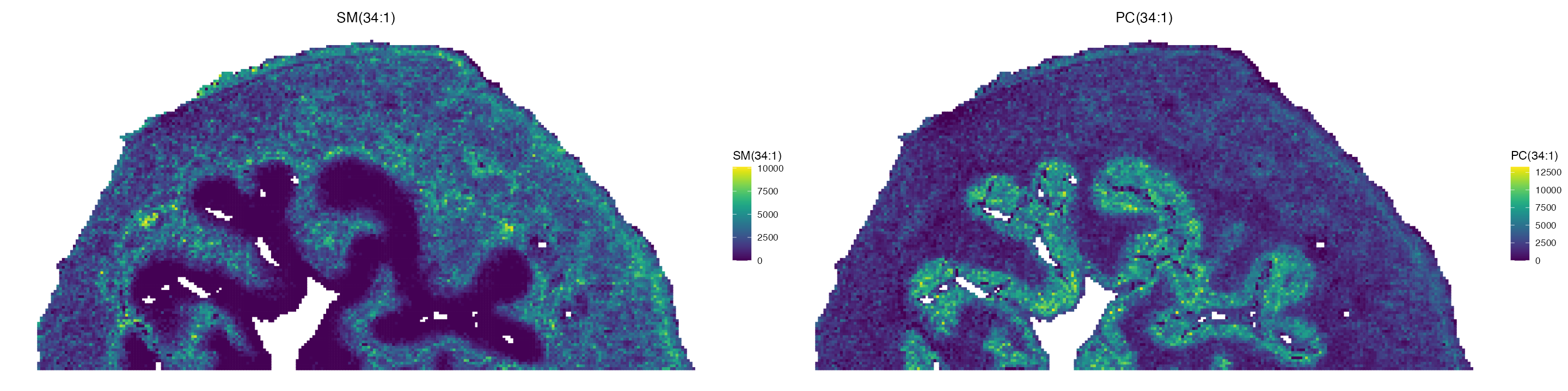
We can see that our annotations match those published previously. Due to the limitations with MSI based technologies, we can not exactly identify the chemical structure of each molecule, meaning that some m/z values have multiple lipid names/annotations.
Differential Expression Analysis of Annotated Metabolites
One key step in understanding biological processes is determining genes, proteins or metabolites that demonstrate significantly different expression between given populations or cell types. Based on the analysis above, for this urinary bladder we identified 3 main tissue regions these being :
| ssc segment | Tissue Region |
|---|---|
| 2 | adventitia |
| 5 | muscle |
| 6 | urothelium |
These regions are identified also in the following references: 1, 2
Lets use SpaMTP’s FindAllDEMs() function to identify differentially expressed m/z metabolites (DEMs) between each of these three tissue regions. This function uses similar methods to those established for genetic data, whereby pixels are pseudo-bulked into random pools and assessed for differential expression (limma.
ROI <- NormalizeSMData(ROI)
# Performs pooling, pseudo-bulking and edgeR Differential Expression Analysis
cluster_DEMs <- FindAllDEMs(data = ROI, slot = "data", ident = "ssc", n = 5, logFC_threshold = 1,
DE_output_dir =NULL, return.individual = FALSE,
run_name = "FindAllDEMs", annotation.column = "all_IsomerNames") # DE results are returned in a data.framePooling one sample into 3 replicates...
Running limma DE Analysis for FindAllDEMs -> with samples [ 5, 2, 6 ]
Starting condition: 5
Starting condition: 2
Starting condition: 6Lets observe the top 10 DE metabolites for each cluster in a heatmap:
DEMsHeatmap(cluster_DEMs, only.pos = FALSE, order.by = "logFC",
plot_annotations_column = "annotations", nlabels.to.show = 1,
n = 15, save_to_path = NULL
,plot.save.height = 10, plot.save.width = 15, annotation_colors = col_palette[c("2","5","6")])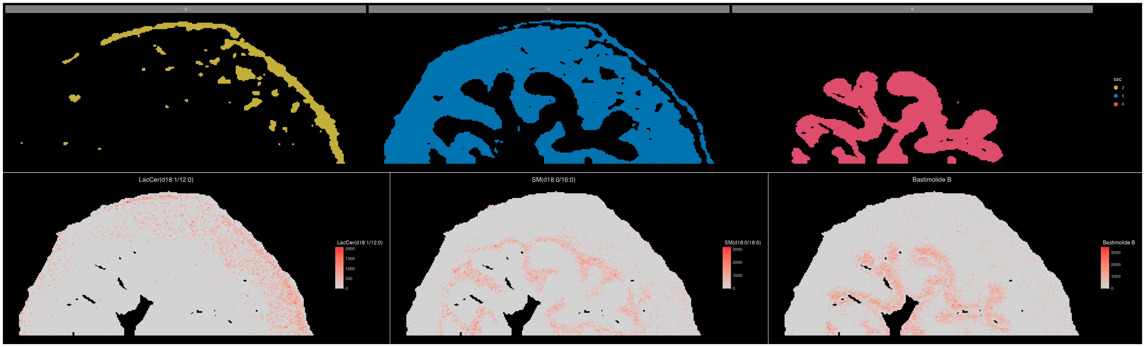
We can also observe the spatial expression patterns of some top DE metabolites.
(ImageDimPlot(ROI, group.by = "ssc", split.by = "ssc", size = 2, cols = col_palette)/
ImageMZAnnotationPlot(ROI, metabolites = c("LacCer(d18:1/12:0)","SM(d18:0/16:0)","Bastimolide B"), size = 2)) & coord_flip() & scale_x_reverse()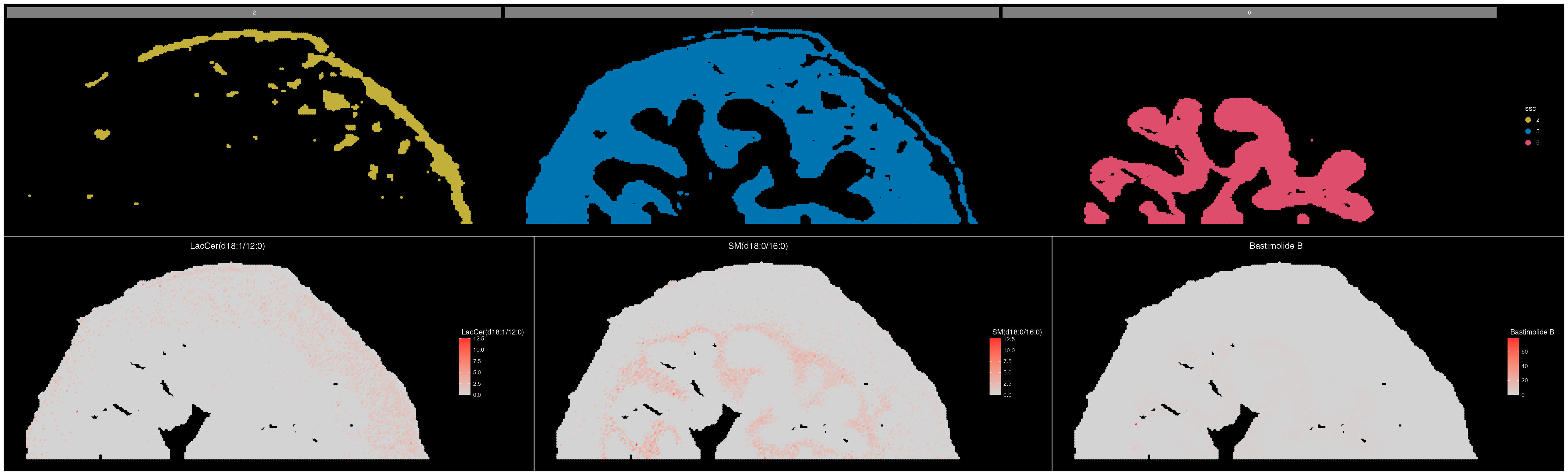
We can see that the expression of these metabolites matches the spatial location of each of these three tissue regions quite well.
Noted in the heatmap above, there are many lipids which are identified as being DE. In particular, there are two lipids of interest which have been identified in the original publication as key metabolites that differentiate the muscle (cluster 5) and urothelium (cluster 6). These being SM(34:1) and PC(34:1) respectively.
The code below performs differential expression analysis just between the the muscle (cluster 5) and urothelium (cluster 6) pixels, to determine if the differential expression of these lipids can be detected.
### Subsets the original dataset to only include cluster 5 and 6
ROI_x <- subset(ROI, subset = ssc %in% c("5", "6"))
### Performs differential expression analysis between the two groups
cluster_DEMs_x <- FindAllDEMs(data = ROI_x, ident = "ssc", n = 5, logFC_threshold = 1,
DE_output_dir =NULL, return.individual = FALSE,
run_name = "FindAllDEMs", annotation.column = "all_IsomerNames" )
### Runs lipid nomenclature simplification on the DEM results
cluster_DEMs_x$DEMs <- RefineLipids(cluster_DEMs_x$DEMs, annotation.column = "annotations", lipid_info = "simple")
### Subsets the DEM results to only get up regulated metabolites for cluster 5 and 6
urothelium <- cluster_DEMs_x$DEMs[cluster_DEMs_x$DEMs$cluster == "6",]
### Sets up colouring for significant spots in volcano plot
keyvals <- ifelse(
urothelium$logFC < 0 & urothelium$P.Value < 10e-4, 'royalblue',
ifelse(urothelium$logFC > 0 & urothelium$P.Value < 10e-4, 'red',
'black'))
keyvals[is.na(keyvals)] <- 'black'
names(keyvals)[keyvals == 'red'] <- 'Cluster 6'
names(keyvals)[keyvals == 'black'] <- 'Non-Sig'
names(keyvals)[keyvals == 'royalblue'] <- 'Cluster 5'
### Changes the shape of the lipid annotations of interest in volcano plot
metabolites <- matches$Species.Name.Simple[1:2]
keyvals.shape <- ifelse(
urothelium$Species.Name.Simple == metabolites[1], 15,
ifelse(urothelium$Species.Name.Simple == metabolites[2], 17,
20))
keyvals.shape[is.na(keyvals.shape)] <- 20
names(keyvals.shape)[keyvals.shape == 20] <- 'Other'
names(keyvals.shape)[keyvals.shape == 15] <- metabolites[1]
names(keyvals.shape)[keyvals.shape == 17] <- metabolites[2]
### Plots volcano plot with DEM results
volc_plot <- EnhancedVolcano::EnhancedVolcano( urothelium,
selectLab = metabolites,
lab = urothelium$Species.Name.Simple,
#FCcutoff = 0,
colCustom = keyvals,
shapeCustom = keyvals.shape,
#cutoffLineType = 'blank',
pCutoff = 10e-4,
FCcutoff = NA,
pointSize = 6,
labSize = 5,
labCol = 'black',
labFace = 'bold',
colAlpha = 4/5,
x = 'logFC',
y = 'P.Value',
gridlines.major = FALSE,
gridlines.minor = FALSE)
volc_plot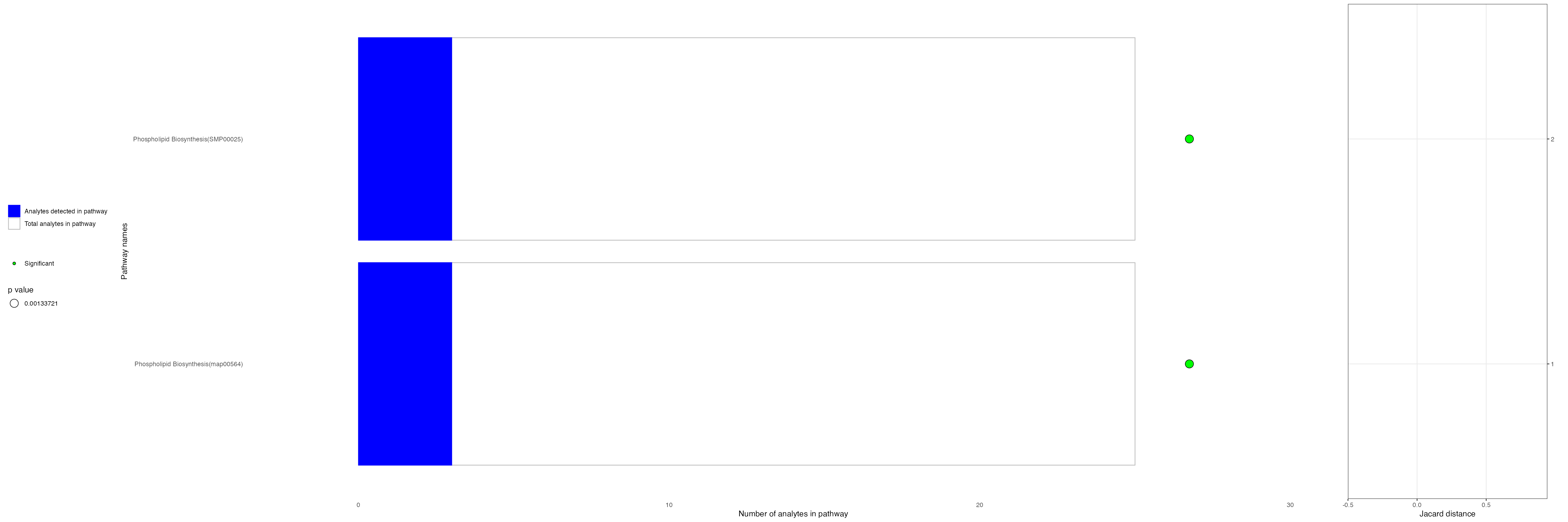
In the volcano plot above, we can see that our analysis correctly identified SM(34:1) to be up-regulated in cluster 5, and PC(34:1) was up-regulated in cluster 6.
Lipids are a key metabolite expressed within the urinary bladder. Lets take a deeper look into the differentially expressed lipids groups with respect to their main category and class:
### Runs lipid nomenclature simplification on the DEM results generated between cluster 2, 5 and 6
cluster_DEMs$DEMs <- RefineLipids(cluster_DEMs$DEMs, annotation.column = "annotations", lipid_info = "simple")
# lets look at the Differenitally expressed Lipids groups
UP <- cluster_DEMs$DEMs[cluster_DEMs$DEMs$regulate == "Up",] # lets get the upregulated lipids for each cluster
# Compute counts of Lipid Maps Categories for 'Up' and 'Down' entries
category_counts <- UP %>%
group_by(cluster, Lipid.Maps.Category) %>%
summarise(count = n()) %>%
ungroup()
category_counts <- category_counts %>%
mutate(Lipid.Maps.Category = ifelse(is.na(Lipid.Maps.Category), "Non-Lipids", Lipid.Maps.Category))
# Plot bar graph
ggplot(category_counts, aes(x = Lipid.Maps.Category, y = count, fill = cluster)) +
geom_bar(stat = "identity", position = "dodge") +
labs(title = "Relative Number of Up Regulated Lipids Grouped by Catagory",
x = "Lipid Maps Category",
y = "Count") +
theme_classic() +
scale_fill_manual(values = col_palette) 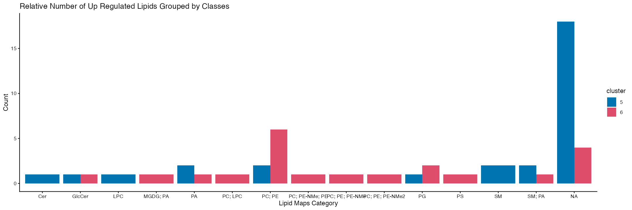
The results displayed in the bar graph above demonstrate the number of different types of lipid categories differentially expressed in each cluster. Lipid categories are the most simple/broad annotation of a lipid. For example, GL stands for glycerolipids, which can represent such lipids classes as diglycerols and triglycerols. Likewise, SP stands for sphingolipids, which include lipids from classes such as sphingomyelins and glycosphingolipids. For more information on different lipid categories and classes, please visit the following links (1,2).
Lets now look at the different lipid classes that were differentially expressed by each cluster.
# Compute counts of Lipid Maps Categories for 'Up' and 'Down' entries
category_counts <- UP %>%
group_by(cluster, Lipid.Maps.Main.Class) %>%
summarise(count = n()) %>%
ungroup()
category_counts <- category_counts %>%
mutate(Lipid.Maps.Category = ifelse(is.na(Lipid.Maps.Main.Class), "Non-Lipids", Lipid.Maps.Main.Class))
# Plot bar graph
ggplot(category_counts, aes(x = Lipid.Maps.Main.Class, y = count, fill = cluster)) +
geom_bar(stat = "identity", position = "dodge") +
labs(title = "Relative Number of Up Regulated Lipids Grouped by Classes",
x = "Lipid Maps Category",
y = "Count") +
theme_classic() +
scale_fill_manual(values = col_palette) 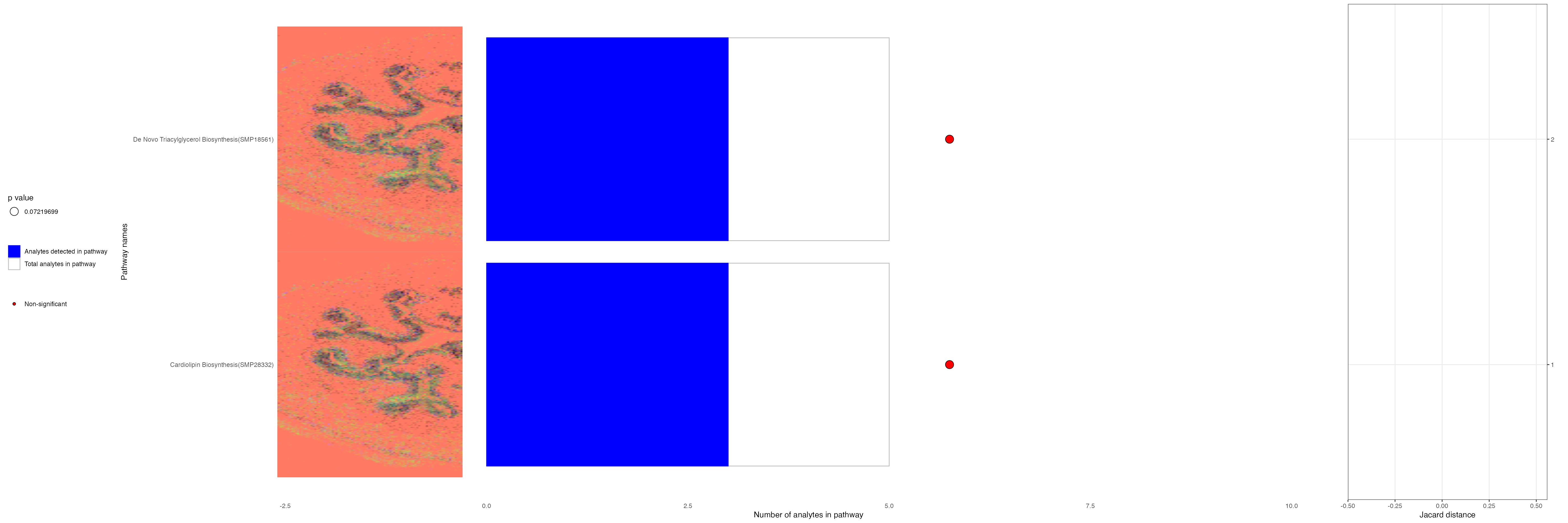
Metabolite Expression Visualisation
Based on the analysis performed above, there are various ways we can visualise the data spatially. SpaMTP has a large range of methods to visualise data including binning common metabolites, 3D plots displaying metabolite/gene expression and more. Below, we will demonstrate some of the key plotting methods.
First, using the DE lipid results from above, we can plot the combined expression of all glycerophospholipids (GP) that were up expressed by our urothelium cells (cluster 6).
### Identified the m/z values that are GP lipids up expressed in cluster 6
mz <- na.omit(UP[c(UP$cluster == "6"& UP$Lipid.Maps.Category == "GP"),]$gene)
### Adds the binned expression value of all of these lipids into a column in the SpaMTP object's @meta.data slot
ROI <- BinMetabolites(ROI, mz, slot = "counts", bin_name = "GPs")
head(ROI, n = 3)| orig.ident | nCount_Spatial | nFeature_Spatial | x_coord | y_coord | sample | ssc | GPs | |
|---|---|---|---|---|---|---|---|---|
| 130_11 | SpaMTP | 70658.19 | 56 | 130 | 11 | mouse-bladder-peaks | 5 | 0.0000 |
| 123_12 | SpaMTP | 50833.22 | 25 | 123 | 12 | mouse-bladder-peaks | 5 | 0.0000 |
| 124_12 | SpaMTP | 60326.05 | 40 | 124 | 12 | mouse-bladder-peaks | 5 | 669.3766 |
ImageFeaturePlot(ROI, features = c("GPs"), size = 2, dark.background = F) & coord_flip() & scale_x_reverse()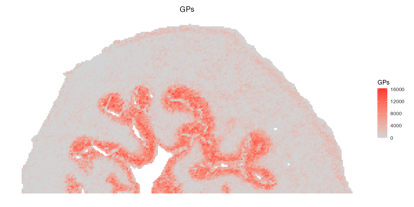
We can see clearly that the combined expression of these GP lipids is highly expressed in the urothelium cells.
Next, we can observe the expression of two key lipids (same as those described above) in a 3D plot:
### Identified the m/z values that are to be plot
mzs <- unlist(lapply(c(798.5411, 741.5306), function(x) FindNearestMZ(data = ROI, target_mz = x)))
Plot3DFeature(ROI, features = mzs, assays = "Spatial", between.layer.height = 100, names = c("PC(34:1)","SM(34:1)"), plot.height = 400, plot.width = 700)Based on our analysis above the lipid ‘PC(30:2)’ was enriched in the uroepithelum cluster (cluster 6). This lipid was not mentioned in the original paper, but may be biologically relevant to the uroepithelum. To check this we can generate some key visualisations:
ImageMZAnnotationPlot(bladder_annotated, metabolites = "PC(30:2)", column.name = "Species.Name.Simple", size = 2) & coord_flip() & scale_x_reverse()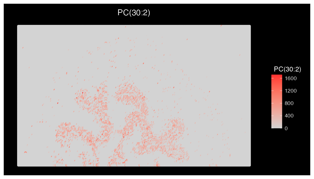
SpaMTP also includes a useful density plot function that generates a HTML which allows the user to simultaneously visualise any m/z peak and it’s relative metabolite annotation spatially. Users have access to a mass intensity plot where they can select any m/z peak, which will then be plotted and all possible metabolite annotations will be listed. Lets demonstrate below, try visualising “mz-740.471557617188” which matches the plot for ‘PC(30:2)’ above:
DensityMap(object = ROI, assay = "Spatial", slot = "counts", folder = "vignette_data_files/Mouse_Urinary_Bladder/")Pathway Analysis
In order to understand biological processes and complex diseases at a deeper level, we often look at biological pathways as a whole rather the expression of just individual metabolites/genes. SpaMTP pathway analysis uses a reference dataset that contains various biological pathways (i.e. KEGG or RAMP_DB) to determine significant changes in biological, cellular or molecular processes.
The first pathway analysis method uses the Fishers Exact Test to identify significant differentially expressed pathways based on the presence of specified features. Users can provide a list of metabolites or metabolites and genes, identified through DE analysis. This method will then identify significant pathways based on the relative proportion of features matching between the list provided and those present within the pathway.
The below code is performing FishersExactTest Pathway analysis on metabolites significantly over expressed in the urothelium (cluster 6):
## Subsets to include only UP-regulated m/z values in cluster 6 (relative to cluster 2 and 5)
cluster_6 <- UP[UP$cluster == "6",]
## Based on these mz values we can get their corresponding annotations which are in the database ID format (stored in `$all_Isomer_IDs`)
metabolite_ids <- ROI[["Spatial"]]@meta.data[ROI[["Spatial"]]@meta.data$all_IsomerNames %in% cluster_6$annotations,]$all_Isomers_IDs
## We can then unlist them to get all the unique possible annotations
metabolite_ids <- unique(unlist(lapply(metabolite_ids, function(x){strsplit(x, "; ")[[1]]})))
### NOTE: Rather then matching the annotation results back to the metabolite annotations, DE can be run changing the 'annotation.column' = "all_Isomer_IDs`Lets now run FishersPathwayTest
cluster_6_pathways <- FishersPathwayAnalysis(list("metabolites" = metabolite_ids),
max_path_size = 500,
alternative = "greater",
min_path_size = 5,
pathway_all_info = T,
pval_cutoff = 0.05,
verbose = TRUE)Fisher Testing ......
Loading files ......
Loading files finished!
Expanding database to extract all potential metabolites
Parsing the information of given analytes class
Begin metabolic pathway analysis ......
Merging datasets
Running test
Calculating p value......
P value obtained
Done
cluster_6_pathways[1:4,]| pathway_name | pathway_id | type | pathwayCategory | p_val | fdr | ratio | analytes_in_pathways | total_in_pathways |
|---|---|---|---|---|---|---|---|---|
| Phospholipid Biosynthesis | SMP00025 | hmdb | smpdb3 | 0.0008121 | 0.0849884 | 0.1200000 | 3 | 25 |
| Phospholipid Biosynthesis | map00564 | kegg | kegg | 0.0008121 | 0.0849884 | 0.1200000 | 3 | 25 |
| Phosphatidylethanolamine Biosynthesis PE(15:0/18:2(9Z,12Z)) | SMP15122 | hmdb | smpdb3 | 0.0036366 | 0.0849884 | 0.1666667 | 2 | 12 |
| Phosphatidylethanolamine Biosynthesis PE(20:1(11Z)/18:3(6Z,9Z,12Z)) | SMP15441 | hmdb | smpdb3 | 0.0036366 | 0.0849884 | 0.1666667 | 2 | 12 |
We can also run FisherPathwayTest using just m/z values. Lets try
this below and see how the results differ. This time we will use
Chebi_db, Lipidmaps_db and
HMDB_db to annotate the m/z values, and we will use all
possible positive adducts. (Note: the mz values are stored in the
data.frame column called gene).
cluster_6_mz_pathways <- FishersPathwayAnalysis(list("mzs" = cluster_6$gene),
min_path_size = 5,
max_path_size = 500,
alternative = "greater",
pathway_all_info = T,
pval_cutoff = 1,
verbose = TRUE)
cluster_6_mz_pathways[1:4,]| pathway_name | pathway_id | type | pathwayCategory | p_val | fdr | ratio | analytes_in_pathways | total_in_pathways |
|---|---|---|---|---|---|---|---|---|
| De Novo Triacylglycerol Biosynthesis TG(18:0/24:1(15Z)/16:1(9Z)) | SMP18561 | hmdb | smpdb3 | 0.0647146 | 0.9184676 | 0.6 | 3 | 5 |
| De Novo Triacylglycerol Biosynthesis TG(18:0/24:1(15Z)/18:0) | SMP18556 | hmdb | smpdb3 | 0.0647146 | 0.9184676 | 0.6 | 3 | 5 |
| De Novo Triacylglycerol Biosynthesis TG(18:0/24:1(15Z)/18:1(9Z)) | SMP18563 | hmdb | smpdb3 | 0.0647146 | 0.9184676 | 0.6 | 3 | 5 |
| De Novo Triacylglycerol Biosynthesis TG(18:0/24:1(15Z)/18:2(9Z,12Z)) | SMP18568 | hmdb | smpdb3 | 0.0647146 | 0.9184676 | 0.6 | 3 | 5 |
Now, lets visualise these results.We will first plot the results generated based on the provided metabolite ID’s.
VisualisePathways(ROI,pathway_df = cluster_6_pathways,p_val_threshold = 0.1,assay = "Spatial",slot = "counts")
We can also plot the results generated from running Fishers Exact Test using the m/z values. This will allow us to plot the expression of each pathway spatially!
VisualisePathways(bladder_annotated,pathway_df = cluster_6_mz_pathways,p_val_threshold = 0.1,assay = "Spatial",slot = "counts")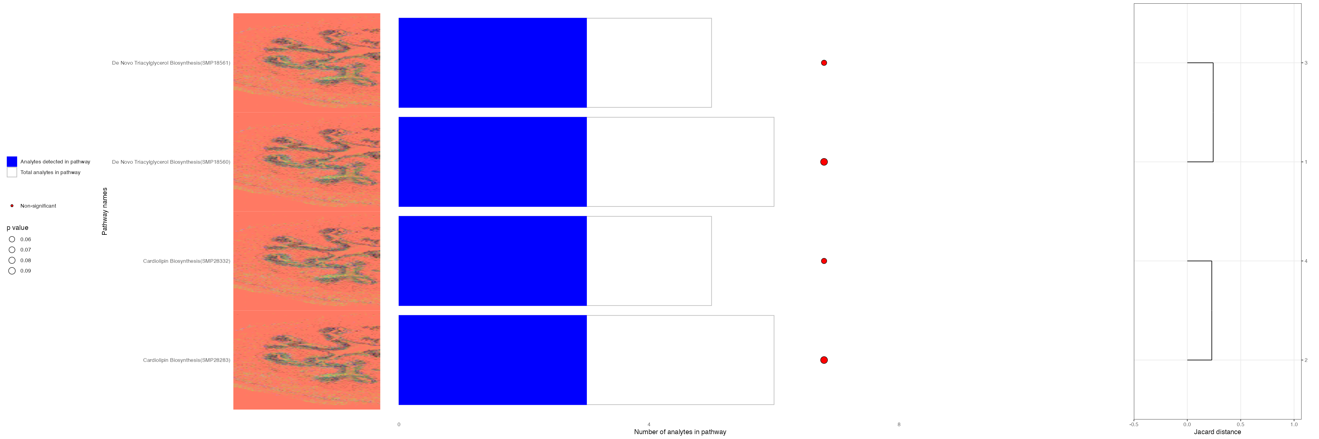
The second form of pathway analysis identifies differentially expressed pathways per group/cluster based on a the relative expression of metabolites and/or genes. Using a similar approach to GSEA features are ranked based on log fold change between groups, and the relative enrichment scores of these features are used to identify significant pathways differentially expressed by each group.
The code below uses the “ssc” clustering and the pseudo-bulking DE results to identify significant pathways per cluster:
DE_pathways <- FindRegionalPathways(SpaMTP = ROI,
ident = "ssc",
DE.list = list(cluster_DEMs$DEMs),
analyte_types = c("metabolites"),
SM_assay = "Spatial",
ST_assay = NULL)
DE_pathways| pathwayName | pval | padj | log2err | ES | NES | size | leadingEdge | Cluster_id | adduct_info | leadingEdge_metabolites | leadingEdge_metabolites_id | leadingEdge_genes | met_regulation | rna_regulation | group_importance | pathwayRampId | sourceId | type | pathwayCategory |
|---|---|---|---|---|---|---|---|---|---|---|---|---|---|---|---|---|---|---|---|
| Fabry disease | 0.5793872 | 0.5793872 | 0.0541201 | 0.3614572 | 0.9085367 | 5 | RAMP_C_0…. | 5 | 682.457092285156[M+K];769.561889648438[M+K] | GlcCer(d18:1/12:0);SM(d18:1/18:0) | LIPIDMAPS:LMSP0501AA01;LIPIDMAPS:LMSP03010001 | ↑;↑ | 9.452459 | RAMP_P_000000110 | SMP00525 | hmdb | smpdb3 | ||
| Gaucher Disease | 0.5793872 | 0.5793872 | 0.0541201 | 0.3614572 | 0.9085367 | 5 | RAMP_C_0…. | 5 | 682.457092285156[M+K];769.561889648438[M+K] | GlcCer(d18:1/12:0);SM(d18:1/18:0) | LIPIDMAPS:LMSP0501AA01;LIPIDMAPS:LMSP03010001 | ↑;↑ | 9.452459 | RAMP_P_000000111 | SMP00349 | hmdb | smpdb3 | ||
| Globoid Cell Leukodystrophy | 0.5793872 | 0.5793872 | 0.0541201 | 0.3614572 | 0.9085367 | 5 | RAMP_C_0…. | 5 | 682.457092285156[M+K];769.561889648438[M+K] | GlcCer(d18:1/12:0);SM(d18:1/18:0) | LIPIDMAPS:LMSP0501AA01;LIPIDMAPS:LMSP03010001 | ↑;↑ | 9.452459 | RAMP_P_000000112 | SMP00348 | hmdb | smpdb3 | ||
| Krabbe disease | 0.5793872 | 0.5793872 | 0.0541201 | 0.3614572 | 0.9085367 | 5 | RAMP_C_0…. | 5 | 682.457092285156[M+K];769.561889648438[M+K] | GlcCer(d18:1/12:0);SM(d18:1/18:0) | LIPIDMAPS:LMSP0501AA01;LIPIDMAPS:LMSP03010001 | ↑;↑ | 9.452459 | RAMP_P_000000113 | SMP00526 | hmdb | smpdb3 | ||
| Metachromatic Leukodystrophy (MLD) | 0.5793872 | 0.5793872 | 0.0541201 | 0.3614572 | 0.9085367 | 5 | RAMP_C_0…. | 5 | 682.457092285156[M+K];769.561889648438[M+K] | GlcCer(d18:1/12:0);SM(d18:1/18:0) | LIPIDMAPS:LMSP0501AA01;LIPIDMAPS:LMSP03010001 | ↑;↑ | 9.452459 | RAMP_P_000000114 | SMP00347 | hmdb | smpdb3 | ||
| Sphingolipid metabolism: integrated pathway | 0.0031260 | 0.0218823 | 0.4317077 | 0.6366434 | 1.9063261 | 8 | RAMP_C_0…. | 5 | 682.457092285156[M+K];741.530578613281[M+K];743.546752929688[M+K];769.561889648438[M+K];825.623657226562[M+K];853.655090332031[M+K] | GlcCer(d18:1/12:0);SM(d18:1/16:0);SM(d18:0/16:0);SM(d18:0/18:1(9Z));SM(d18:1/22:0);SM(d18:1/24:0) | LIPIDMAPS:LMSP0501AA01;LIPIDMAPS:LMSP03010003;LIPIDMAPS:LMSP03010004;LIPIDMAPS:LMSP03010031;LIPIDMAPS:LMSP03010006;LIPIDMAPS:LMSP03010008 | ↑;↑;↑;↑;↑;↑;↑ | 9.452459 | RAMP_P_000053493 | WP4726 | wiki | NA | ||
| Sphingolipid metabolism: integrated pathway | 0.0008139 | 0.0008139 | 0.4772708 | -0.7352415 | -2.0949124 | 7 | RAMP_C_0…. | 6 | 682.457092285156[M+K];741.530578613281[M+K];743.546752929688[M+K];769.561889648438[M+K];825.623657226562[M+K];853.655090332031[M+K] | GlcCer(d18:1/12:0);SM(d18:1/16:0);SM(d18:0/16:0);SM(d18:0/18:1(9Z));SM(d18:1/22:0);SM(d18:1/24:0) | LIPIDMAPS:LMSP0501AA01;LIPIDMAPS:LMSP03010003;LIPIDMAPS:LMSP03010004;LIPIDMAPS:LMSP03010031;LIPIDMAPS:LMSP03010006;LIPIDMAPS:LMSP03010008 | ↓;↓;↓;↓;↓;↓;↓ | 9.452459 | RAMP_P_000053493 | WP4726 | wiki | NA | ||
| Starch and sucrose metabolism | 0.5793872 | 0.5793872 | 0.0541201 | 0.3614572 | 0.9085367 | 5 | RAMP_C_0…. | 5 | 682.457092285156[M+K];769.561889648438[M+K] | GlcCer(d18:1/12:0);SM(d18:1/18:0) | LIPIDMAPS:LMSP0501AA01;LIPIDMAPS:LMSP03010001 | ↑;↑ | 9.452459 | RAMP_P_000000115 | map00500 | kegg | kegg |
Based on this, we can see that there is only one significant
differentially expressed pathway. Before we annotated our sample based
on only M+K analytes, and using the LIPIDMAPS database. To
increase the number of possible pathways detected we can broaden our
annotation range to include M+H and M+K
analytes from the HMDB, LIPIDMAPS and ChEBI databases and re-run the
analysis.
## Get Data
ROI_pathays <- subset(bladder, subset = ssc %in% c("2", "5", "6"))
## Re-annotate
ROI_pathays <- AnnotateSM(ROI_pathays, db = rbind(Chebi_db,Lipidmaps_db,HMDB_db), ppm_error = 15, polarity = "positive", adducts = c("M+H","M+K"))
## Re-run DE analysis
DE <- FindAllDEMs(data = ROI_pathays, ident = "ssc", n = 5, logFC_threshold = 1,
DE_output_dir =NULL, return.individual = FALSE,
run_name = "FindAllDEMs", annotation.column = "all_IsomerNames")
DE_pathways <- FindRegionalPathways(SpaMTP = ROI_pathays,
ident = "ssc",
DE.list = list(DE$DEMs),
analyte_types = c("metabolites"),
SM_assay = "Spatial",
ST_assay = NULL)
DE_pathways| pathwayName | pval | padj | log2err | ES | NES | size | leadingEdge | Cluster_id | adduct_info | leadingEdge_metabolites | leadingEdge_metabolites_id | leadingEdge_genes | met_regulation | rna_regulation | group_importance | pathwayRampId | sourceId | type | pathwayCategory |
|---|---|---|---|---|---|---|---|---|---|---|---|---|---|---|---|---|---|---|---|
| Fabry disease | 0.7328340 | 0.7540574 | 0.0383206 | 0.3131984 | 0.8000280 | 6 | RAMP_C_0…. | 5 | 567.053955078125[M+H];682.457092285156[M+K];756.549621582031[M+H];769.561889648438[M+K];844.525817871094[M+K] | UDP-D-glucose;GlcCer(d18:1/12:0);PC(14:0/20:3(8Z,11Z,14Z));SM(d18:1/18:0);LacCer(d18:1/12:0) | chebi:18066;LIPIDMAPS:LMSP0501AA01;LIPIDMAPS:LMGP01011374;LIPIDMAPS:LMSP03010001;hmdb:HMDB0004866 | ↑;↑;↑;↑;↑ | 10.61282 | RAMP_P_000000110 | SMP00525 | hmdb | smpdb3 | ||
| Gaucher Disease | 0.7328340 | 0.7540574 | 0.0383206 | 0.3131984 | 0.8000280 | 6 | RAMP_C_0…. | 5 | 567.053955078125[M+H];682.457092285156[M+K];756.549621582031[M+H];769.561889648438[M+K];844.525817871094[M+K] | UDP-D-glucose;GlcCer(d18:1/12:0);PC(14:0/20:3(8Z,11Z,14Z));SM(d18:1/18:0);LacCer(d18:1/12:0) | chebi:18066;LIPIDMAPS:LMSP0501AA01;LIPIDMAPS:LMGP01011374;LIPIDMAPS:LMSP03010001;hmdb:HMDB0004866 | ↑;↑;↑;↑;↑ | 10.61282 | RAMP_P_000000111 | SMP00349 | hmdb | smpdb3 | ||
| Globoid Cell Leukodystrophy | 0.7328340 | 0.7540574 | 0.0383206 | 0.3131984 | 0.8000280 | 6 | RAMP_C_0…. | 5 | 567.053955078125[M+H];682.457092285156[M+K];756.549621582031[M+H];769.561889648438[M+K];844.525817871094[M+K] | UDP-D-glucose;GlcCer(d18:1/12:0);PC(14:0/20:3(8Z,11Z,14Z));SM(d18:1/18:0);LacCer(d18:1/12:0) | chebi:18066;LIPIDMAPS:LMSP0501AA01;LIPIDMAPS:LMGP01011374;LIPIDMAPS:LMSP03010001;hmdb:HMDB0004866 | ↑;↑;↑;↑;↑ | 10.61282 | RAMP_P_000000112 | SMP00348 | hmdb | smpdb3 | ||
| Krabbe disease | 0.7328340 | 0.7540574 | 0.0383206 | 0.3131984 | 0.8000280 | 6 | RAMP_C_0…. | 5 | 567.053955078125[M+H];682.457092285156[M+K];756.549621582031[M+H];769.561889648438[M+K];844.525817871094[M+K] | UDP-D-glucose;GlcCer(d18:1/12:0);PC(14:0/20:3(8Z,11Z,14Z));SM(d18:1/18:0);LacCer(d18:1/12:0) | chebi:18066;LIPIDMAPS:LMSP0501AA01;LIPIDMAPS:LMGP01011374;LIPIDMAPS:LMSP03010001;hmdb:HMDB0004866 | ↑;↑;↑;↑;↑ | 10.61282 | RAMP_P_000000113 | SMP00526 | hmdb | smpdb3 | ||
| Metachromatic Leukodystrophy (MLD) | 0.7328340 | 0.7540574 | 0.0383206 | 0.3131984 | 0.8000280 | 6 | RAMP_C_0…. | 5 | 567.053955078125[M+H];682.457092285156[M+K];756.549621582031[M+H];769.561889648438[M+K];844.525817871094[M+K] | UDP-D-glucose;GlcCer(d18:1/12:0);PC(14:0/20:3(8Z,11Z,14Z));SM(d18:1/18:0);LacCer(d18:1/12:0) | chebi:18066;LIPIDMAPS:LMSP0501AA01;LIPIDMAPS:LMGP01011374;LIPIDMAPS:LMSP03010001;hmdb:HMDB0004866 | ↑;↑;↑;↑;↑ | 10.61282 | RAMP_P_000000114 | SMP00347 | hmdb | smpdb3 | ||
| Sphingolipid metabolism | 0.1028417 | 0.1028417 | 0.1596467 | -0.6463355 | -1.3866096 | 5 | RAMP_C_0…. | 2 | 503.981231689453[M+H];558.094543457031[M+K];567.053955078125[M+H];784.528564453125[M+K] | ATP(4-);MP-A08;UDP-D-glucose;PE(14:0/22:1(13Z)) | chebi:30616;chebi:167665;chebi:18066;hmdb:HMDB0008842 | ↓;↓;↓;↓ | 10.61282 | RAMP_P_000049972 | map00600 | kegg | kegg | ||
| Sphingolipid metabolism | 0.1028417 | 0.1028417 | 0.1596467 | -0.6463355 | -1.3866096 | 5 | RAMP_C_0…. | 2 | 503.981231689453[M+H];558.094543457031[M+K];567.053955078125[M+H];784.528564453125[M+K] | ATP(4-);MP-A08;UDP-D-glucose;PE(14:0/22:1(13Z)) | chebi:30616;chebi:167665;chebi:18066;hmdb:HMDB0008842 | ↓;↓;↓;↓ | 10.61282 | RAMP_P_000050230 | R-HSA-428157 | reactome | NA | ||
| Sphingolipid metabolism | 0.1028417 | 0.1028417 | 0.1596467 | -0.6463355 | -1.3866096 | 5 | RAMP_C_0…. | 2 | 503.981231689453[M+H];558.094543457031[M+K];567.053955078125[M+H];784.528564453125[M+K] | ATP(4-);MP-A08;UDP-D-glucose;PE(14:0/22:1(13Z)) | chebi:30616;chebi:167665;chebi:18066;hmdb:HMDB0008842 | ↓;↓;↓;↓ | 10.61282 | RAMP_P_000053711 | WP2788 | wiki | NA | ||
| Sphingolipid metabolism | 0.7540574 | 0.7540574 | 0.0369933 | 0.3079555 | 0.7866357 | 6 | RAMP_C_0…. | 5 | 503.981231689453[M+H];558.094543457031[M+K];567.053955078125[M+H];686.583801269531[M+K];703.57470703125[M+H];742.533813476562[M+H] | ATP(4-);MP-A08;UDP-D-glucose;Cer(d18:1/24:1(15Z));SM(d18:0/16:1(9Z));PE(18:3(9Z,12Z,15Z)/18:0) | chebi:30616;chebi:167665;chebi:18066;LIPIDMAPS:LMSP02010009;hmdb:HMDB0013464;LIPIDMAPS:LMGP02010720 | ↑;↑;↑;↑;↑;↑ | 10.61282 | RAMP_P_000049972 | map00600 | kegg | kegg | ||
| Sphingolipid metabolism | 0.7540574 | 0.7540574 | 0.0369933 | 0.3079555 | 0.7866357 | 6 | RAMP_C_0…. | 5 | 503.981231689453[M+H];558.094543457031[M+K];567.053955078125[M+H];686.583801269531[M+K];703.57470703125[M+H];742.533813476562[M+H] | ATP(4-);MP-A08;UDP-D-glucose;Cer(d18:1/24:1(15Z));SM(d18:0/16:1(9Z));PE(18:3(9Z,12Z,15Z)/18:0) | chebi:30616;chebi:167665;chebi:18066;LIPIDMAPS:LMSP02010009;hmdb:HMDB0013464;LIPIDMAPS:LMGP02010720 | ↑;↑;↑;↑;↑;↑ | 10.61282 | RAMP_P_000050230 | R-HSA-428157 | reactome | NA | ||
| Sphingolipid metabolism | 0.7540574 | 0.7540574 | 0.0369933 | 0.3079555 | 0.7866357 | 6 | RAMP_C_0…. | 5 | 503.981231689453[M+H];558.094543457031[M+K];567.053955078125[M+H];686.583801269531[M+K];703.57470703125[M+H];742.533813476562[M+H] | ATP(4-);MP-A08;UDP-D-glucose;Cer(d18:1/24:1(15Z));SM(d18:0/16:1(9Z));PE(18:3(9Z,12Z,15Z)/18:0) | chebi:30616;chebi:167665;chebi:18066;LIPIDMAPS:LMSP02010009;hmdb:HMDB0013464;LIPIDMAPS:LMGP02010720 | ↑;↑;↑;↑;↑;↑ | 10.61282 | RAMP_P_000053711 | WP2788 | wiki | NA | ||
| Sphingolipid metabolism: integrated pathway | 0.0353688 | 0.2829504 | 0.3217759 | 0.5268847 | 1.5870626 | 10 | RAMP_C_0…. | 5 | 682.457092285156[M+K];703.57470703125[M+H];743.546752929688[M+K];769.561889648438[M+K];825.623657226562[M+K];851.640014648438[M+K];853.655090332031[M+K] | GlcCer(d18:1/12:0);SM(d18:1/16:0);SM(d18:0/16:0);SM(d18:1/18:0);N-docosanoylsphingosine-1-phosphocholine;beta-D-glucosyl-(1<->1’)-N-[(15Z)-tetracosenoyl]sphinganine;SM(d18:1/24:0) | LIPIDMAPS:LMSP0501AA01;LIPIDMAPS:LMSP03010003;LIPIDMAPS:LMSP03010004;LIPIDMAPS:LMSP03010001;chebi:74532;chebi:84699;LIPIDMAPS:LMSP03010008 | ↑;↑;↑;↑;↑;↑;↑;↑ | 10.61282 | RAMP_P_000053493 | WP4726 | wiki | NA | ||
| Sphingolipid metabolism: integrated pathway | 0.0011822 | 0.0011822 | 0.4550599 | -0.7266723 | -2.0523438 | 8 | RAMP_C_0…. | 6 | 682.457092285156[M+K];703.57470703125[M+H];769.561889648438[M+K];825.623657226562[M+K];851.640014648438[M+K];853.655090332031[M+K] | GlcCer(d18:1/12:0);SM(d18:1/16:0);SM(d18:1/18:0);N-docosanoylsphingosine-1-phosphocholine;beta-D-glucosyl-(1<->1’)-N-[(15Z)-tetracosenoyl]sphinganine;SM(d18:1/24:0) | LIPIDMAPS:LMSP0501AA01;LIPIDMAPS:LMSP03010003;LIPIDMAPS:LMSP03010001;chebi:74532;chebi:84699;LIPIDMAPS:LMSP03010008 | ↓;↓;↓;↓;↓;↓;↓ | 10.61282 | RAMP_P_000053493 | WP4726 | wiki | NA | ||
| Starch and sucrose metabolism | 0.7328340 | 0.7540574 | 0.0383206 | 0.3131984 | 0.8000280 | 6 | RAMP_C_0…. | 5 | 567.053955078125[M+H];682.457092285156[M+K];756.549621582031[M+H];769.561889648438[M+K];844.525817871094[M+K] | UDP-D-glucose;GlcCer(d18:1/12:0);PC(14:0/20:3(8Z,11Z,14Z));SM(d18:1/18:0);LacCer(d18:1/12:0) | chebi:18066;LIPIDMAPS:LMSP0501AA01;LIPIDMAPS:LMGP01011374;LIPIDMAPS:LMSP03010001;hmdb:HMDB0004866 | ↑;↑;↑;↑;↑ | 10.61282 | RAMP_P_000000115 | map00500 | kegg | kegg |
We can see that we now have many more differentially expressed pathways! Lets plot these results:
PlotRegionalPathways(regpathway = DE_pathways)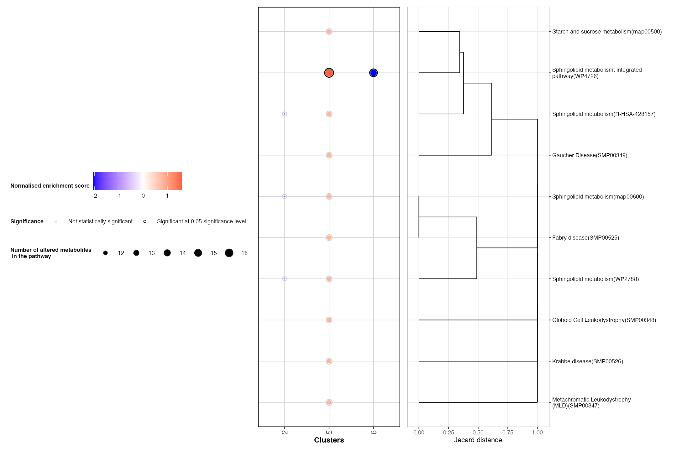
This plot highlights that cluster 5 (bladder muscle) is enriched for
Biochemical pathways. Alternatively, the urothelium
(cluster 6) is shown to down regulate numerous pathways including
Sphingolipid metabolism. This matches with previous
research suggesting that the metabolism of sphingolipids is mainly
associated with muscle cells of the badder.
These results may not tell the entire story however, the ‘SSC’ clustering results do not capture every region of the tissue according to the original publication. There is a specific area between the bladder and urothelium called the ‘lamina propria’ which is currently unidentifiable based on the ‘SSC’ clustering result (this was also mentioned in the original paper).
Clustering using PCA and Seurat
Because SpaMTP is built on the foundations of a Seurat Object, it allows the user to still use many useful Seurat functions on their spatial metabolomic data using SpaMTP. Below, we will demonstrate how to use metabolite-based PCA results from SpaMTP, along with Seurat’s clustering functions, to identify this rare cell type known as the (lamina propria).
First we will run clustering:
ROI <- RunMetabolicPCA(ROI, assay = "Spatial", slot = "counts")
ROI <- FindNeighbors(ROI, dims = 1:30, verbose = FALSE) # use the SpaMTP object generated from PCA Pathway Analysis
ROI <- RunUMAP(ROI, dims = 1:30, verbose = FALSE)
ROI <- FindClusters(ROI, resolution = 0.3, cluster.name = "clusters", verbose = FALSE)Now, lets plot the results:
## Custom palette for SpaMTP/Seurat Clustering
SpaMTP_palette = list("0" = "#0074B0",
"1" = "#008E87",
"2" = "#DE4D6C",
"3" = "#BF212E",
"4" = "#C2B03B" ,
"5" = "#92f09a",
"6" = "#9FBEAC")
DimPlot(ROI, group.by = "clusters", cols = SpaMTP_palette, pt.size = 2) | ImageDimPlot(ROI, size = 2, group.by = "clusters", cols = SpaMTP_palette) + coord_flip() + scale_x_reverse()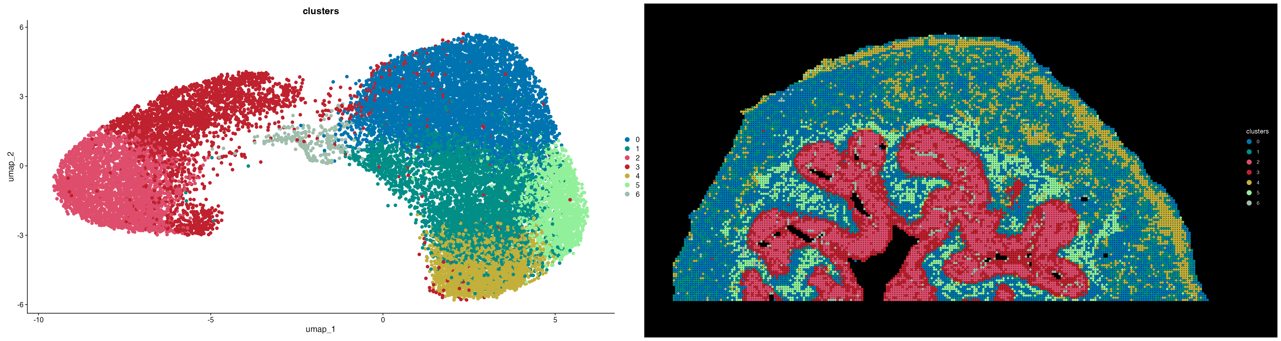
Comparing these results to the SSC segmentation we can see this clustering can still detect the urinary bladder muscle (cluster 0/1), urothelium (cluster 2/3) and the adventitia (cluster 4). In addition, we are able to detect a region that matches a similar location to that of the lamina propria (cluster 5) identified by the original publication.
Finding Spatially Correlated Metabolites
An added benefit of using spatial technologies rather then single-cell/bulk methods is the retainment of spatial context. This allows us to analyse trends across the whole tissue section that would otherwise be lost in bulk analyses.
In the original publication they defined an m/z = 743.5482 as the lamina propria.
Lets use SpaMTP’s feature co-localisation function to check the top metabolites that spatially correlate to cluster 5!
correlated_features <- FindCorrelatedFeatures(ROI, ident = "clusters", SM.assay = "Spatial", nfeatures = 6) #find the spatial correlation between each cluster and their relative metabolitesBecause we are interested in the lamina propria, lets focus on the top correlated metabolites with cluster 5:
df <- correlated_features[correlated_features$ident == "5",] # subsets to only include results from cluster 5
df$mz_name <- paste0("mz-",round(df$mz, digits = 6)) # simplifies the m/z names for the plot
## Plots the top 10 results
ggplot(df, aes(x = -rank, y = correlation)) + geom_bar(stat = "identity") + geom_text(aes(label = mz_name), vjust = -0.5, size = 3, color = "black") + coord_flip() + theme_classic()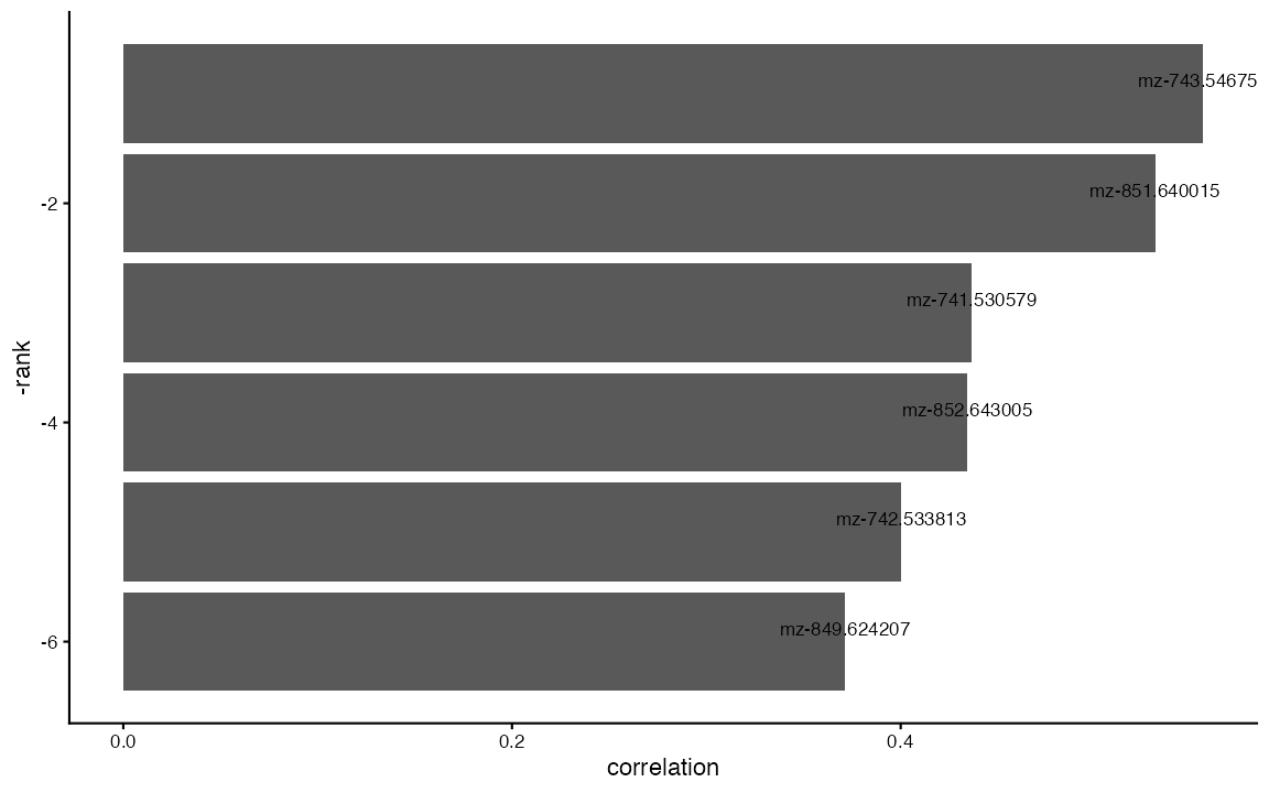
We can see that our top hit is m/z = 734.5467, which is described in Cardinal’s paper as the peak defining the lamina propria.
We can check by looking at the spatial expression of this m/z:
## Formats Plots
plots <- list()
for (i in c("0", "2", "3", "4", "5")){
suppressWarnings(clst <- subset(ROI, subset = clusters %in% i))
plots[[i]] <- ImageDimPlot(clst, group.by = "clusters", cols = SpaMTP_palette, size = 1.5)
}
plots[["mz"]] <- ImageFeaturePlot(ROI, features = 'mz-743.546752929688', size = 1.2) & scale_fill_gradientn(colors = viridis::turbo(100))
## Plots data
patchwork::wrap_plots(plots, ncol = 3, nrow = 2)& coord_flip() & scale_x_reverse()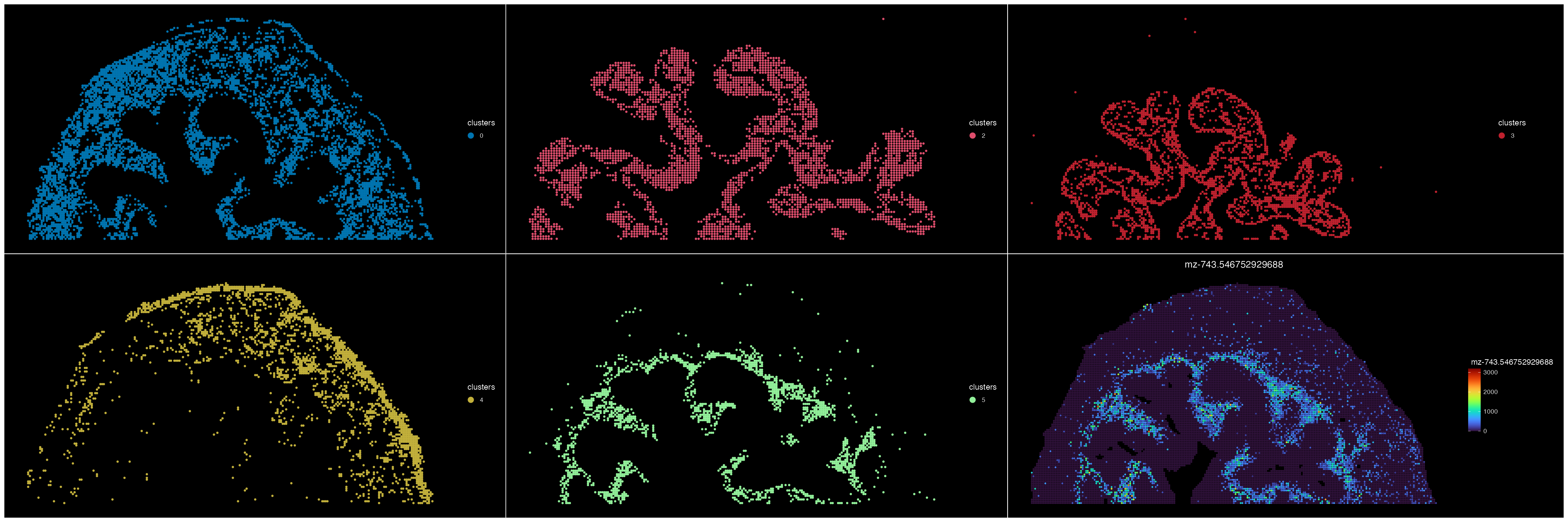
In addition to finding correlated m/z’s based on spatial location, we can also identify metabolites that demonstrate a strong spatial pattern. This is done using Moran’s I scores to determine the most spatially variable features.
ROI <- FindSpatiallyVariableMetabolites(ROI, assay = "Spatial", image = "fov") # Finds Spatially Strong m/z's
ImageFeaturePlot(ROI, features = GetSpatiallyVariableMetabolites(ROI, assay = "Spatial", n = 6), size = 1) & coord_flip() & scale_x_reverse()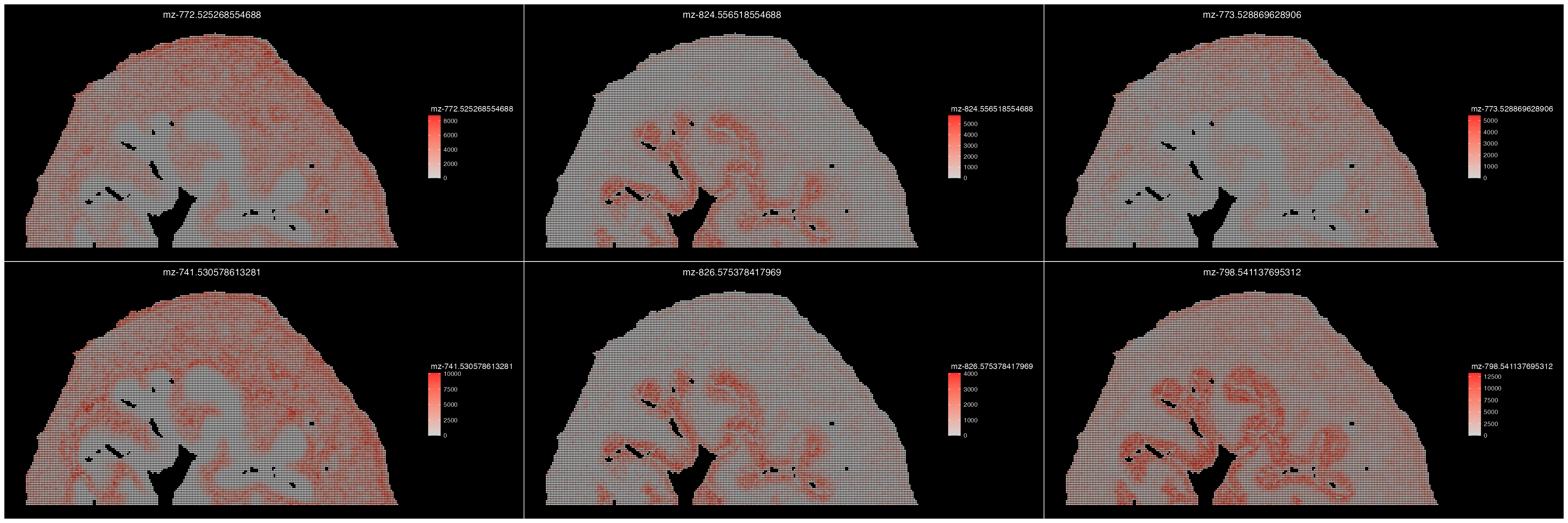
Switching between SpaMTP and Cardinal Objects
Similar to before we can interchangeably convert our data between SpaMTP and Cardinal objects, meaning pre-processing or analysis tools from either package can be used at any point during the analysis pipeline.
As an example, we can convert our SpaMTP object to Cardinal to generate a figure overlaying key m/z values. Lets first convert our data:
bladder_cardinal <- ConvertSeuratToCardinal(data = ROI, assay = "Spatial", slot = "counts")Gathering Intensity, m/z values and metadata from Seurat Object ...
Converting intensity matrix and Generating Cardinal Object ...
bladder_cardinal## MSImagingExperiment with 79 features and 21164 spectra
## spectraData(1): intensity
## featureData(1): mz
## pixelData(13): x, y, run, ..., Seurat_metadata.GPs, Seurat_metadata.clusters, Seurat_metadata.seurat_clusters
## coord(2): x = 9...247, y = 11...134
## runNames(1): run0
## mass range: 426.9289 to 970.1479
## centroided: NAWe can see that the Object layout is correct and we have 79 annotated
m/z values and our seurat metadata has also been stored in the
pixelData slot. Next we can generate a plot using
Cardinal:
image(bladder_cardinal, mz=c(798.5410, 741.5307, 743.5482),
main="Mouse urinary bladder",
col=c("red", "lightblue", "green"),
contrast.enhance="suppress",
smooth.image="adaptive",
normalize.image="linear",
superpose=TRUE)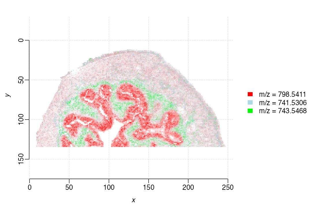
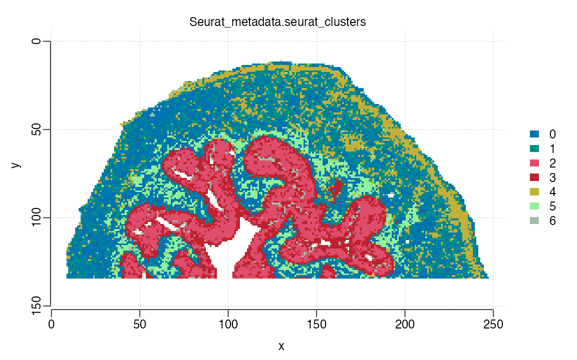 We can see based on this ion image overlay plot that the three selected
m/z values correspond quite significantly with our
Seurat based clustering. 743.5482 clearly maps cluster 5
(green), whereas 798.5410 corresponds to cluster 2 and 3 (red).
We can see based on this ion image overlay plot that the three selected
m/z values correspond quite significantly with our
Seurat based clustering. 743.5482 clearly maps cluster 5
(green), whereas 798.5410 corresponds to cluster 2 and 3 (red).
Additional Pathway Analysis
We can also run pathway analysis on the new clustering results. Lets
do that now, this time using Seurat’s
FindAllMarker() function to calculating DE metabolites,
highlighting SpaMTP’s flexibility. You will
see below that FindAllMarker() requires normalised data.
SpaMTP has a NormalizeSMData()
function that allows for TIC (Total Ion Current) normalisation.
For more info on this form of normalisation, please read Jauhiainen et.al
(2014).
## Annotate ROI with additional datasets
ROI <- AnnotateSM(ROI, db = rbind(Chebi_db,Lipidmaps_db, HMDB_db), polarity = "positive")
## Performs TIC normalisation
ROI <- NormalizeSMData(ROI)
## Run FindAllMarkers() on clustering results
Idents(ROI) <- "clusters"
DE <- FindAllMarkers(ROI, assay = "Spatial")
## Runs Pathway Analysis between clusters
DE_pathways <- FindRegionalPathways(SpaMTP = ROI,
ident = "clusters",
DE.list = list(DE),
analyte_types = c("metabolites"),
SM_assay = "Spatial",
ST_assay = NULL)Below, we will visualise the top 5 pathways differentially expressed between clusters:
PlotRegionalPathways(regpathway = DE_pathways, num_display = 4)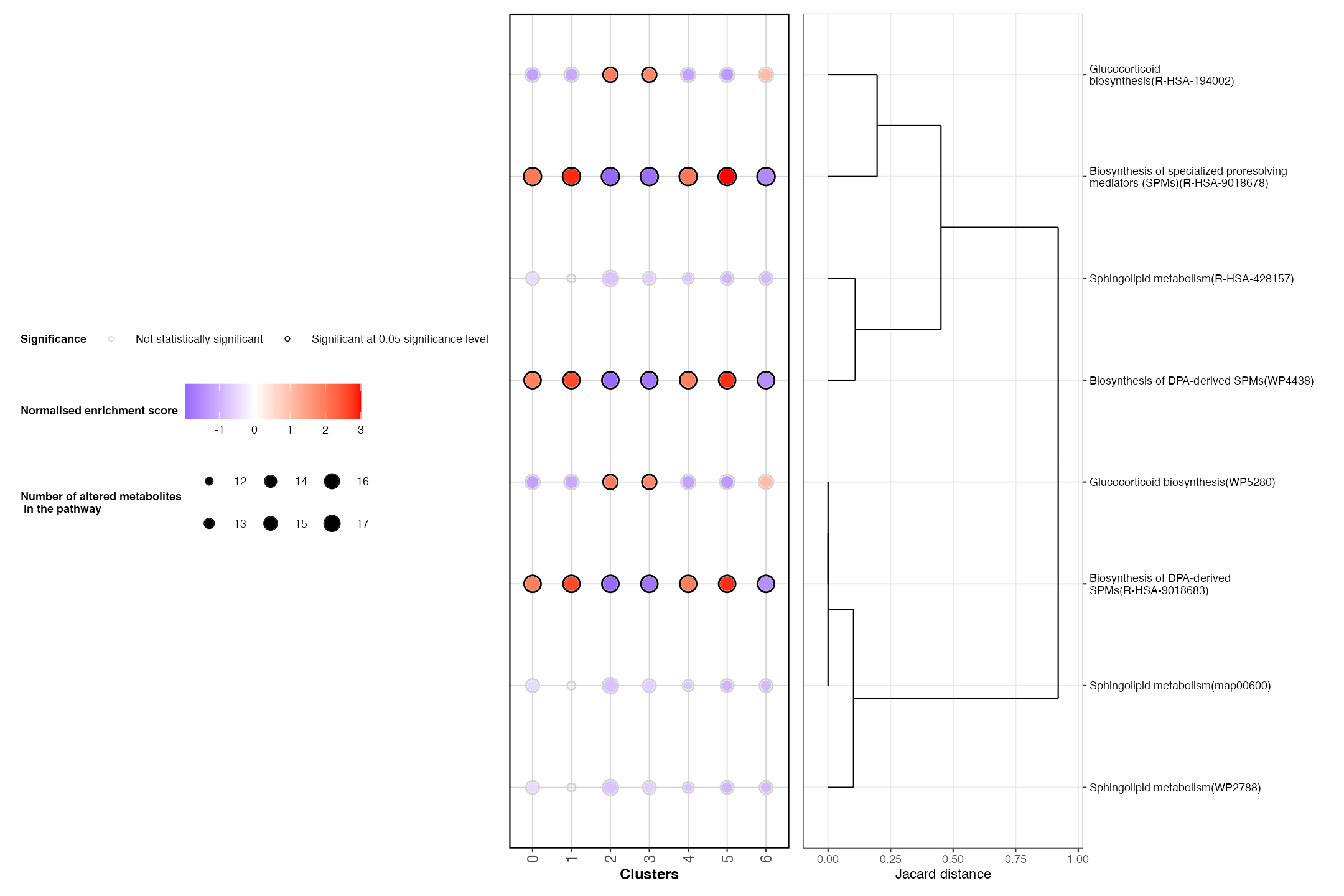
We can also plots some key pathways of interest that were also upregulated in our dataset.
key_pathways <- c("Biochemical pathways: part I","G alpha (i) signalling events","Metabolism of carbohydrates","Sphingolipid metabolism: integrated pathway",
"Sensory perception of sweet, bitter, and umami (glutamate) taste", "Sensory perception of taste",
"G alpha (i) signaling events")
PlotRegionalPathways(regpathway = DE_pathways, selected_pathways = key_pathways)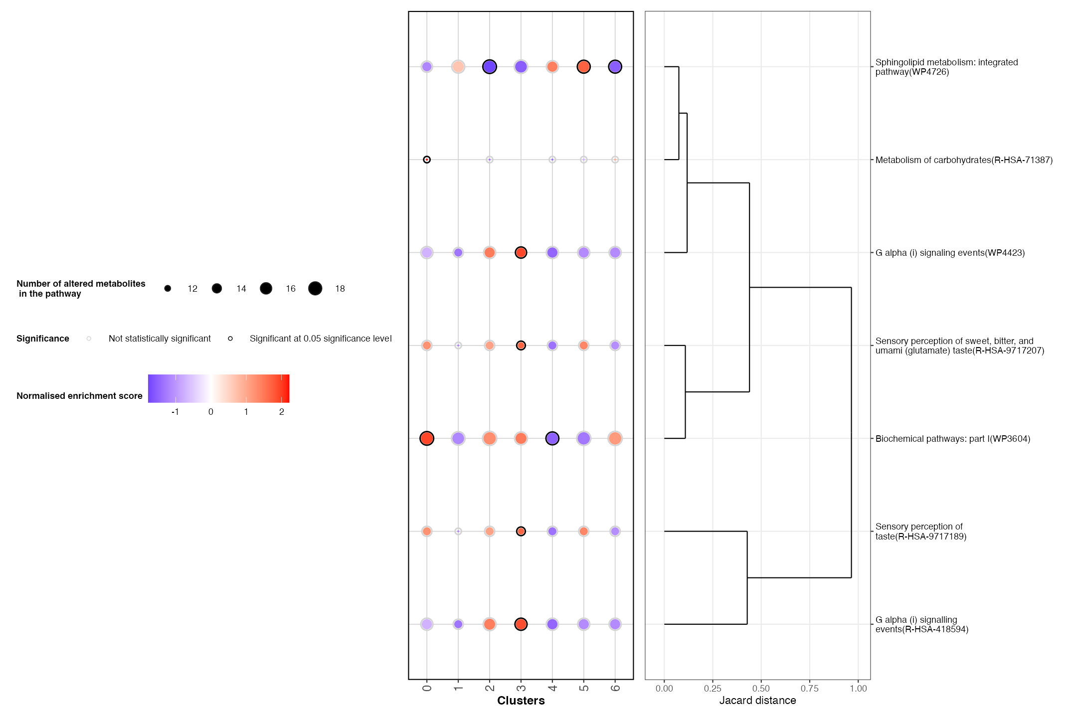
Based on these findings, we observe that the lamina propria (cluster 5) has an up regulation of metabolites associated with sensory perception pathways. This matches with biology, as this is the layer of the bladder that contains sensory neurons.
There are a large range of additional applications SpaMTP can be used for, such as, multi-modality analysis using both spatial transcriptomics and spatial metabolomics. Check out the SpaMTP github or documentation site for more.
Session Info
## R version 4.4.1 (2024-06-14)
## Platform: aarch64-apple-darwin20
## Running under: macOS 15.5
##
## Matrix products: default
## BLAS: /Library/Frameworks/R.framework/Versions/4.4-arm64/Resources/lib/libRblas.0.dylib
## LAPACK: /Library/Frameworks/R.framework/Versions/4.4-arm64/Resources/lib/libRlapack.dylib; LAPACK version 3.12.0
##
## locale:
## [1] en_US.UTF-8/en_US.UTF-8/en_US.UTF-8/C/en_US.UTF-8/en_US.UTF-8
##
## time zone: Europe/Oslo
## tzcode source: internal
##
## attached base packages:
## [1] stats4 stats graphics grDevices utils datasets methods
## [8] base
##
## other attached packages:
## [1] future_1.67.0 kableExtra_1.4.0 knitr_1.50
## [4] htmltools_0.5.8.1 viridis_0.6.5 viridisLite_0.4.2
## [7] EnhancedVolcano_1.24.0 ggrepel_0.9.6 ggplot2_4.0.0
## [10] dplyr_1.1.4 Seurat_5.3.0 SeuratObject_5.2.0
## [13] sp_2.2-0 Cardinal_3.8.3 S4Vectors_0.44.0
## [16] ProtGenerics_1.38.0 BiocGenerics_0.52.0 BiocParallel_1.40.2
## [19] SpaMTP_1.1.0
##
## loaded via a namespace (and not attached):
## [1] fs_1.6.6 matrixStats_1.5.0
## [3] spatstat.sparse_3.1-0 bitops_1.0-9
## [5] sf_1.0-21 EBImage_4.48.0
## [7] httr_1.4.7 RColorBrewer_1.1-3
## [9] tools_4.4.1 sctransform_0.4.2
## [11] R6_2.6.1 lazyeval_0.2.2
## [13] uwot_0.2.3 withr_3.0.2
## [15] gridExtra_2.3 progressr_0.16.0
## [17] cli_3.6.5 Biobase_2.66.0
## [19] textshaping_1.0.3 spatstat.explore_3.5-3
## [21] fastDummies_1.7.5 shinyjs_2.1.0
## [23] labeling_0.4.3 sass_0.4.10
## [25] S7_0.2.0 spatstat.data_3.1-8
## [27] proxy_0.4-27 ggridges_0.5.7
## [29] pbapply_1.7-4 pkgdown_2.1.3
## [31] systemfonts_1.2.3 svglite_2.2.1
## [33] scater_1.34.1 parallelly_1.45.1
## [35] Rfast2_0.1.5.4 CardinalIO_1.4.0
## [37] limma_3.62.2 rstudioapi_0.17.1
## [39] generics_0.1.4 ica_1.0-3
## [41] spatstat.random_3.4-2 crosstalk_1.2.2
## [43] Matrix_1.7-4 ggbeeswarm_0.7.2
## [45] abind_1.4-8 lifecycle_1.0.4
## [47] yaml_2.3.10 edgeR_4.4.2
## [49] SummarizedExperiment_1.36.0 SparseArray_1.6.2
## [51] Rtsne_0.17 grid_4.4.1
## [53] promises_1.3.3 crayon_1.5.3
## [55] miniUI_0.1.2 lattice_0.22-7
## [57] beachmat_2.22.0 cowplot_1.2.0
## [59] zeallot_0.2.0 pillar_1.11.1
## [61] fgsea_1.32.4 GenomicRanges_1.58.0
## [63] future.apply_1.20.0 codetools_0.2-20
## [65] Rnanoflann_0.0.3 fastmatch_1.1-6
## [67] glue_1.8.0 spatstat.univar_3.1-4
## [69] data.table_1.17.8 vctrs_0.6.5
## [71] png_0.1-8 spam_2.11-1
## [73] gtable_0.3.6 zigg_0.0.2
## [75] cachem_1.1.0 xfun_0.53
## [77] S4Arrays_1.6.0 mime_0.13
## [79] Rfast_2.1.5.1 survival_3.8-3
## [81] SingleCellExperiment_1.28.1 pheatmap_1.0.13
## [83] units_0.8-7 statmod_1.5.0
## [85] fitdistrplus_1.2-4 ROCR_1.0-11
## [87] nlme_3.1-168 matter_2.8.0
## [89] RcppAnnoy_0.0.22 GenomeInfoDb_1.42.3
## [91] bslib_0.9.0 irlba_2.3.5.1
## [93] vipor_0.4.7 KernSmooth_2.23-26
## [95] DBI_1.2.3 ggrastr_1.0.2
## [97] tidyselect_1.2.1 compiler_4.4.1
## [99] ontologyIndex_2.12 BiocNeighbors_2.0.1
## [101] xml2_1.4.0 desc_1.4.3
## [103] ggdendro_0.2.0 DelayedArray_0.32.0
## [105] plotly_4.11.0 scales_1.4.0
## [107] classInt_0.4-11 lmtest_0.9-40
## [109] tiff_0.1-12 stringr_1.5.2
## [111] digest_0.6.37 goftest_1.2-3
## [113] fftwtools_0.9-11 spatstat.utils_3.2-0
## [115] rmarkdown_2.29 XVector_0.46.0
## [117] pkgconfig_2.0.3 jpeg_0.1-11
## [119] MatrixGenerics_1.18.1 fastmap_1.2.0
## [121] rlang_1.1.6 htmlwidgets_1.6.4
## [123] UCSC.utils_1.2.0 shiny_1.11.1
## [125] farver_2.1.2 jquerylib_0.1.4
## [127] zoo_1.8-14 jsonlite_2.0.0
## [129] BiocSingular_1.22.0 RCurl_1.98-1.17
## [131] magrittr_2.0.4 scuttle_1.16.0
## [133] GenomeInfoDbData_1.2.13 dotCall64_1.2
## [135] patchwork_1.3.2 Rcpp_1.1.0
## [137] ggnewscale_0.5.2 reticulate_1.43.0
## [139] stringi_1.8.7 zlibbioc_1.52.0
## [141] MASS_7.3-65 plyr_1.8.9
## [143] rgoslin_1.10.0 parallel_4.4.1
## [145] listenv_0.9.1 deldir_2.0-4
## [147] splines_4.4.1 tensor_1.5.1
## [149] locfit_1.5-9.12 igraph_2.1.4
## [151] spatstat.geom_3.6-0 RcppHNSW_0.6.0
## [153] reshape2_1.4.4 ScaledMatrix_1.14.0
## [155] evaluate_1.0.5 RcppParallel_5.1.11-1
## [157] httpuv_1.6.16 RANN_2.6.2
## [159] tidyr_1.3.1 purrr_1.1.0
## [161] polyclip_1.10-7 scattermore_1.2
## [163] rsvd_1.0.5 xtable_1.8-4
## [165] e1071_1.7-16 RSpectra_0.16-2
## [167] later_1.4.4 class_7.3-23
## [169] ragg_1.5.0 tibble_3.3.0
## [171] beeswarm_0.4.0 IRanges_2.40.1
## [173] cluster_2.1.8.1 globals_0.18.0